Yu-Dong Wang
, Jian-Xiong Wang
, Institute of High Energy Physics, Chinese Academy of Sciences, Beijing 100049, China
School of Physics, University of Chinese Academy of Sciences, Beijing 100049, China
Received Date:2018-12-24
Available Online:2019-04-01
Abstract:At the designed circular electron-positron collider (CEPC), similar to the hadron collider, the angular distribution coefficients of the decay lepton pair from the produced Z(W) boson in $ e^+ e^- $ collisions are predicted. Their dependence on cos$ \theta_Z $ (cos$ \theta_W $) are presented in four different polarization frames. Furthermore, the value of the angular distribution coefficients in different bins of cos$ \theta_Z $ are presented in the C-S frame. In comparison with the case at the hadron collider, better accurate measurement for Z(W) is expected because there is less background, and W could be reconstructed from its leptonic decay channel. This works provides a method to precisely test the electroweak production mechanism or some effect induced from new physics in the future measurements at the CEPC.

HTML

--> --> -->

The Drell-Yan process, first proposed in Ref. [1], studies the angular distribution of the lepton pair from the vector boson decay, which is produced in hadron-hadron collisions. For the simplest case, it is predicted that the differential cross section is proportional to $ 1+\cos^2\theta $ at the lowest order when the vector boson is a virtual photon. With the emission and absorption of partons with large transverse momentum, there is a factor of 2 enhancement to the total cross section [2], and the angular distribution becomes more general [3-5]. By measuring the angular distribution coefficients of the final-state lepton, many theoretical works such as the violation of Lam-Tung relation [6] and the forward-backward asymmetry of lepton pair productions [7] were studied.
The Drell-Yan type processes provide a powerful method to understand the production mechanism of the gauge boson and to explore the new physics. In 1983, W and Z boson were discovered [8, 9], and some measurements were found to be consistent with the predictions of the V-A Standard Model [10-12]. The measurement of the angular distribution coefficients of the lepton pair in Z/$ \gamma^* $ production was first reported for $ p\bar{p} $ collisions at 1.96 TeV by CDF Collaboration [13], and the results were found to be in good agreement with the predictions of QCD fixed-order perturbation theory. The measurements were also performed in the CMS and ATLAS collaborations at $ \sqrt{s} $=8 TeV [14-18]. Meanwhile, many theoretical studies have been conducted on the prediction of the inclusive Z boson production, which involves the emission of partons of large transverse momenta [19, 20].
The circular electron-positron collider (CEPC) is proposed to be built in the future. It is designed such that the center-of-mass (CM) energy has a maximum energy of 240 GeV and a higher luminosity than the linear collider [21]; this will have less background compared with the hadron collider. The CEPC project aims to precisely test the properties of the Higgs, Z, and W boson, and investigate new physics. Compared with the process at the hadron collider, a similar process, $e^++e^-\to Z/\gamma^*(W)+X \to $$ l^+l^- (l^-\bar{\nu}_l)+X $, is of interest and should be studied.
In this study, we investigate the angular distribution coefficients of Z boson inclusive production. In comparison with the Z boson hadroproduction, the energy of a Z boson is fixed at leading-order (LO) at $ e^+e^- $ collider. Thus, for a detailed study, we present these angular distribution coefficients dependence on cos$ \theta_Z $ (cos$ \theta_W $); $ \theta_Z $ ($ \theta_W $) is the polar angle of Z(W) boson in the laboratory frame.
The angular differential cross section can be written as

$\frac{{\rm d}\sigma}{{\rm d}\cos\theta_Z {\rm d}\Omega}=\sum_{\lambda \lambda^\prime}\frac{{\rm d}\sigma_{\lambda \lambda^\prime}}{{\rm d}\cos\theta_Z}f_{\lambda \lambda^\prime}(\theta, \varphi),$

(1)

where $ \theta $ and $ \varphi $ are polar and azimuthal angles of the lepton in the Z(W) rest frame, respectively, and $ {\rm d}\Omega={\rm d}\cos\theta {\rm d}\varphi $. $ {\rm d}\sigma_{\lambda \lambda^\prime} $ and $ f_{\lambda \lambda^\prime} $ are the production density matrix of process $ e^+ +e^-\to $$ Z/\gamma^*+X $ and decay density matrix of $Z /\gamma^*\to l^++l^- $, respectively.
The remainder of this paper is organized as follows. In Section 2, we present the general expression of the lepton angular distribution of this process. We also represent the angular coefficients by the gauge boson production density matrix elements. In Section 3, we numerically calculate the angular distribution coefficients for the total and differential cross section in different polarization frames. In Section 4, we present the figures of the angular coefficients of Z(W) production dependence on cos$ \theta_Z $ (cos$ \theta_W $). In addition, the coefficients of Z production processes are calculated at different bins of cos$ \theta_Z $. Finally, the summary and conclusion are provided in Section 5.

For simplicity, we focus on the Z boson production and the situation is same for W boson. In $e^+(p_1)+e^-(p_2) \to $$ Z(p_Z)+X(p_X) \to $$ l^+(k_1) + l^- (k_2)+ X(p_X) $ (l is $ \mu $ or e), two planes must be defined, which are named as the production plane and the decay plane. In the lab frame, as shown in Fig. 1, the first one is formed by the beam direction and $ \vec{p}_{Z} $; the angle between them is $ \theta_Z $. The other plane is formed by $ \vec{p}_{Z} $ and $ \vec{k}_{1} $, the corresponding angle in the Z boson rest frame is $ \theta $. Finally, the angle between the production and the decay plane is $ \varphi $, which is invariant under the Lorentz transformation, from the lab frame to the Z-rest frame.
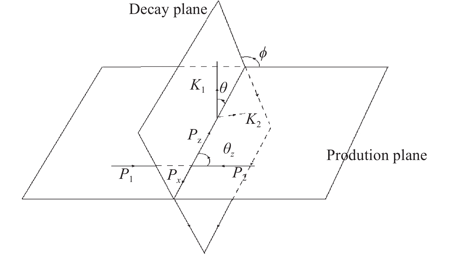Figure1. Production and decay planes and various angles in lab frame.

The dilepton angular distribution is defined in the Z boson rest frame, and we use this frame in the following discussion. The invariant mass window of Z boson is chosen at approximately 91.19 GeV. The total cross section can be represented as

$\begin{split}\sigma & = (M_{\gamma^*}+M_z)(M_{\gamma^*}+M_z)^*\\ & = |M_{\gamma^*}|^2+|M_z|^2+2{\rm Re}(M_{\gamma^*}M_z^*)\\ & = \sigma_{\gamma^*}+\sigma_z+\sigma_{\gamma^* z}, \end{split}$

(2)

where $ M_{\gamma^*} $ and $ M_z $ represent the amplitude of $ \gamma^* $ and Z boson mediate parts, respectively. See Eq. (5), the amplitude of these parts are proportional to $ 1/({p^2-m^2-im\Gamma }) $. Then, the value of $ \sigma_{\gamma^*}/\sigma_z $ and $ \sigma_{\gamma^* z}/\sigma_z $ are estimated to be $ \Gamma_z^2/m_z^2 $ and $ \Gamma_z/m_z $ (where $ \Gamma_Z $ is the decay width of Z boson), respectively. The uncertainty produced by $ \sigma_{\gamma^*} $ and $ \sigma_{\gamma^* z} $ is estimated to be approximately 2.8% in the following calculation where only$ \sigma_z $ is keeped.
To obtain a more precision estimation, the cross section for $ e^+ e^- \to Z/\gamma^* +X \to l^+ l^-+X $ and $ e^+ e^- \to Z +X \to l^+ l^-+$$ X $ are calculated in the region $ (m_z-\Gamma_z/2)^2 <(k_1+k_2)^2 < $$ (m_z+\Gamma_z/2)^2 $. The value of $ (\sigma_{\gamma^*}+\sigma_{\gamma^* z})/\sigma_z $ was obtained as 0.43%, 0.69%, and 2.38%, where X is a photon, Z boson, and Higgs, respectively. When the proportion of the cross section of the ZH channel in the total cross section is approximately 0.42%, then the total uncertainty from $ \sigma_{\gamma^*} $ and $ \sigma_{\gamma^* z} $ is less than 1%. Therefore, the calculation in this study did not consider the effect of $ \gamma^* $ mediate part.
The momentum of Z boson, $ l^- $, and $ l^+ $ at Z boson rest frame are expressed as

$\begin{split}& p_Z =(E, 0, 0, 0), \\ & k_1 =\frac{E}{2}(1, \sin \theta \cos\varphi, \sin\theta \sin\varphi, \cos\theta), \\ & k_2 =\frac{E}{2}(1, -\sin\theta \cos\varphi, -\sin\theta \sin\varphi, -\cos\theta), \end{split}$

(3)

where the mass of the fermion (mass of $ e, \mu, u, ... $) is set to zero approximately. There are four commonly used polarization frames [22] that correspond to different choices for the Z-axis, which are the recoil (helicity) frame ($ \vec{Z}\!=\!-\displaystyle\frac{\vec{p}_{1}+\vec{p}_{2}}{|\vec{p}_{1}+\vec{p}_{2}|} $), Gottfried-Jackson frame ($ \vec{Z}=\displaystyle\frac{\vec{p}_{2}}{|\vec{p}_{2}|} $), target frame ($ \vec{Z}=-\displaystyle\frac{\vec{p}_{1}}{|\vec{p}_{1}|} $), and the Collins-Soper(C-S) [23] ($ \vec{Z}\propto \displaystyle\frac{\vec{p}_{1}}{|\vec{p}_{1}|}+\displaystyle\frac{\vec{p}_{2}}{|\vec{p}_{2}|} $). The $ \vec{p}_{1} $ and $ \vec{p}_2 $ is in the Z boson rest frame. The C-S frame was frequently used in the measurements in the hadron collision. For example, the polarization vector in the helicity frame is expressed as

$\epsilon_\pm=\left(0, \mp\frac{1}{\sqrt{2}}, -\frac{i}{\sqrt{2}}, 0\right), \epsilon_0=(0, 0, 0, 1).$

(4)

The amplitude of each channel ($ X_i $) in inclusive Z boson production can be written as

$\begin{split}M_i & = M_{e^+e^-\to ZX_i}^\mu \frac{-i\left(g_{\mu \nu}-\displaystyle\frac{p_{z\mu} p_{z\nu}}{m_z^2+im_z\Gamma }\right) }{p_z^2-m_z^2-im_z\Gamma_z}M_{Z\to l^+l^-}^\nu \\ & = \sum_\lambda M_{e^+e^-\to ZX_i}^\mu \frac{\epsilon_{\lambda\mu} \epsilon^*_{\lambda\nu}}{m_z\Gamma_z} M_{Z\to l^+l^-}^\nu = \sum_\lambda a_{\lambda}(X_i)\frac{1}{m_z \Gamma_z}b_\lambda, \end{split}$

(5)

where $ a_\lambda (X_i)=M_{e^++e^-\to Z+X_i}^\mu \epsilon_{\lambda\mu} $ and $ b_\lambda =\epsilon^*_{\lambda\nu}M_{Z\to l^+l^-}^\nu $. Both $ a_\lambda (X_i) $ and $ b_\lambda $ are Lorentz invariant. Therefore they can be calculated in different frames. $ a_\lambda (X_i) $ and $ b_\lambda $ are calculated in the lab frame and the Z boson rest frame, respectively. The production and decay density matrix are defined as

$\begin{split}& \sigma_{\lambda \lambda^{\prime}}= \sum_ia_\lambda (X_i) a_{\lambda^\prime}^*(X_i), \\ & D_{\lambda \lambda^{\prime}} = \sum_{s_1, s_2}b_\lambda b_{\lambda^\prime}^*, \\ & b_\lambda = \bar{\mu}(k_2, s_2)(ig_v \gamma_\mu+ig_a \gamma_\mu \gamma_5)\nu(k_1, s_1) \epsilon_\lambda^*, \end{split}$

(6)

where the decay density matrix $ D_{\lambda \lambda^{\prime}} $ can be obtained easily, and the production matrix $ \sigma_{\lambda \lambda^{\prime}} $ is discussed in Appendix A.
By applying $ D_{\lambda \lambda^{\prime}} $ and $ \sigma_{\lambda \lambda^{\prime}} $, the differential cross section is expressed as [4]

$\begin{split}\frac{{\rm d}\sigma}{{\rm d}\Omega}& \propto (g_v^2+g_a^2)Sp^2(1+\lambda_{\theta}\cos^2\theta \\ + &\lambda_{\varphi}\sin^2\theta \cos(2\varphi)+\lambda_{\theta \varphi}\sin(2\theta) \cos\varphi \\ + &\lambda_{\varphi}^\bot \sin^2\theta \sin(2\varphi)+\lambda_{\theta \varphi}^\bot \sin(2\theta) \sin\varphi \\ + &\alpha_{\theta} \cos\theta+\alpha_{\theta \varphi} \sin\theta \cos\varphi +\alpha_{\theta \varphi}^{ \bot } \sin\theta \sin\varphi), \end{split}$

(7)

where $ \theta $ and $ \varphi $ are the polar and azimuthal angles of the dilepton in Z boson rest frame, respectively. The coefficients of each term are given below

$\begin{split}& S = {\sigma _{ + + }} + {\sigma _{ - - }} + 2{\sigma _{00}}, \\ & {\lambda _\theta } = \frac{{{\sigma _{ + + }} + {\sigma _{ - - }} - 2{\sigma _{00}}}}{S}, \;\;\;\;\;\;\;\;\;\;{\lambda _\varphi } = \frac{{2{\rm Re}({\sigma _{ - + }})}}{S}, \\ & \lambda _\varphi ^ \bot = \frac{{ - 2{\rm Im}({\sigma _{ - + }})}}{S}, \;\;\;\;\;\;\;\;\;\;\;\;\;\;\;\;\;\;\;\;{\lambda _{\theta \varphi }} = \frac{{\sqrt 2 {\rm Re}({\sigma _{ + 0}} - {\sigma _{ - 0}})}}{S}, \\ & \lambda _{\theta \varphi }^ \bot = \frac{{\sqrt 2 {\rm Im}({\sigma _{ + 0}} + {\sigma _{ - 0}})}}{S}, \;\;\;\;\;\;\;\;{\alpha _\theta } = \frac{{ - 2{A_l}({\sigma _{ + + }} - {\sigma _{ - - }})}}{S}, \\ & {\alpha _{\theta \varphi }} = \frac{{2\sqrt 2 {A_l}{\rm Re}({\sigma _{ + 0}} + {\sigma _{ - 0}})}}{S}, \;\;\alpha _{\theta \varphi }^ \bot = \frac{{2\sqrt 2 {A_l}{\rm Im}({\sigma _{ + 0}} - {\sigma _{ - 0}})}}{S}.\end{split}$

(8)

The asymmetry parameter of fermion f is $ A_f= \displaystyle\frac{2g_v g_a}{g^2_v+g^2_a} $, as given in PDG [24]; its value are 0.1515±0.0019 and 0.142±0.015 for electron and muon, respectively. In this study, $ A_l $= 0.1515 is used. From Eq. (8), there are additional three terms, $ \alpha_\theta $, $ \alpha_{\theta \varphi} $, and $ \alpha_{\theta \varphi}^\bot $ compared to the case in which $ J/\Psi $ production decay to the lepton pair [25] owing to the presence of parity-violation coupling $ g_a $. When $ g_a=0 $, these terms disappear. From the above expressions, $ \lambda_{\varphi}^{\bot} $, $ \lambda_{\theta\varphi}^{\bot} $, and $ \alpha_{\theta\varphi}^{\bot} $, which are proportional to sin$ \varphi $ or sin2$ \varphi $, come from the contributions of the imaginary part of the density matrix elements.
As presented in Appendix A, there are relations Eq. (A5) for the real part in $ \sigma_{\lambda \lambda^\prime} $, which are caused by the coupling $ g_v $. According to Eq. (8), this part does not contribute to the values of $ \alpha_\theta $ and $ \alpha_{\theta \varphi} $. Meanwhile $\displaystyle\frac{g_a}{g_v}= $$ \frac{1-\sqrt{1-A_f^2}}{A_f} $= 0.076, the contribution of the imaginary part, proportional to $ g_a $, is small. It is expected that the values of $ \alpha_\theta $ and $ \alpha_{\theta \varphi} $ are much smaller than the other coefficients. In particular, the following relations are obtained:

$\begin{split} & - 1 \leqslant {\lambda _\theta } \leqslant 1, \;\;\;\;\;\;\;\;\;\;\;\;\;\;\;\;\;\;\;\;\, - 1 \leqslant {\lambda _\varphi } \leqslant 1, \\ & \frac{{ - 1}}{{\sqrt 2 }} \leqslant {\lambda _{\theta \varphi }} \leqslant \frac{1}{{\sqrt 2 }}, \;\;\;\;\;\;\;\;\;\;\;\;\; - 2{A_l} \le {\alpha _\theta } \leqslant 2{A_l}, \\ & - \sqrt 2 {A_l} \leqslant {\alpha _{\theta \varphi }} \leqslant \sqrt 2 {A_l}, \;\;\; - 1 \leqslant \lambda _\varphi ^ \bot \leqslant 1, \\ & \frac{{ - 1}}{{\sqrt 2 }} \leqslant \lambda _{\theta \varphi }^ \bot \leqslant \frac{1}{{\sqrt 2 }}, \;\;\;\;\;\;\;\;\;\;\;\;\;\; - \sqrt 2 {A_l} \leqslant \alpha _{\theta \varphi }^ \bot \leqslant \sqrt 2 {A_l}, \end{split}$

(9)

At LO, the production of the Z boson come from the following three processes

$\begin{split}& e^+ +e^- \to Z + \gamma \to l^+ +l^- + \gamma, \\ & e^+ +e^- \to Z + Z \to l^+ +l^- + Z, \\ & e^+ +e^- \to Z + H \to l^+ +l^- + H.\end{split}$

(10)

The production density matrices of the Z boson in these processes are calculated using the package FDC [26], and the values of the angular distribution coefficients are obtained.
In these three processes, the $ Z \gamma $ production have a larger contribution in the cross section compared with others. The cross section are 46.64 pb, 0.96 pb, and 0.20 pb for $ Z\gamma $, ZZ, and ZH production channels, respectively. Summed up all above production channels, the value of dilepton angular distribution coefficients at Z pole are shown in the Table 1. The total cross section refer to the inclusive Z boson production $ e^+ +e^- \to Z + X $. The differential cross section denpendence on $\mathrm{cos}\theta_Z$($\mathrm{cos}\theta_W$) for each channel and their sum are also given in the Fig. 2.

cos$ \theta_Z $	$ \lambda_\theta $	$ \lambda_\varphi $	$ \lambda_{\theta \varphi} $	$ \alpha_\theta $	$ \alpha_{\theta\varphi} $	$ \lambda_{\varphi}^\bot $	$ \lambda_{\theta \varphi}^\bot $	$ \alpha_{\theta \varphi}^\bot $	Total cross section(pb)
cos$ \theta_Z $>0	0.937	0.008	0.030	0.031	?0.0003	0	0	0	23.90
cos$ \theta_Z $<0	0.937	0.008	?0.030	?0.031	?0.003	0	0	0	23.90
total	0.937	0.008	0	0	?0.003	0	0	0	47.80

Table1.Values of angular distribution coefficients and total cross section for Z boson productions at $ \sqrt{s} $=240 GeV in the Recoil frame.

Figure2. (color online) Differential cross section of Z(W) boson production.

The cross section is much smaller compared with the Drell-Yan type process in hadron collisions [27] at LO; to obtain accurate measurements, larger integrated luminosity is required. From the CEPC design report [21], at the CM energy $ \sqrt{s}=240 $ GeV, the luminosity of the CEPC is approximately 3×10³⁴ cm^?1s^?1. The integrated value is approximately 0.8 ab^?1/year (it operates for about 8 months, each year), the total number of Z bosons produced each year is approxiamtely 3.82×10⁷. It is expected to run for 7 years at this energy, according to the fraction of the Z decay modes [24]. The total events of the electron and muon pairs should be 1.80×10⁷. In addition, the events of the jets, if we use the jets to reconstruct Z boson, is approximately 1.87×10⁸. In ATLAS [18], the total events of lepton pair is approximately 1.25×10⁷, it is closed to the value at the CEPC. Moreover, there is less background at the CEPC. Therefore, a good accuracy is expected in future CEPC experiments in the measurement of angular distribution coefficients in inclusive Z boson production.
The value of $ \lambda_\varphi^\bot $, $ \lambda_{\theta \varphi}^\bot $, and $ \alpha_{\theta \varphi}^\bot $ are all 0. These terms are proportional to the imaginary part of the density matrix elements in Eq. (8). In the calculations, the imaginary part of the density matrix is zero at LO, and these terms will not be discussed hereinafter. However, for Z boson production at the hadron collider [6], these coefficients are nonzero at next-to-leading order (NLO) corrections in QCD.
From Table 1, the values of $ \lambda_{\theta \varphi} $ and $ \alpha_\theta $ are 0 when the full range of cos$ \theta_Z $ is considered because they are antisymmetric in value for cos$ \theta_Z> 0 $ and cos$ \theta_Z < 0 $. Usually, there is a Lam-Tung [3] relation for the coefficients $ \lambda_\theta $ and $ \lambda_\varphi $. In the Drell-Yan process, $ 1-\lambda_\theta =4 \lambda_\varphi $, with the vector boson in the gauge invariant condition (i.e., virtual photon) for the full final state phase space (except the dilepton) integration. For the electroweak interaction in this situation, we found that $ \lambda_\theta+4\lambda_\varphi $ is approximately equal to 0.97. It does not obey the relation like the mediate virtual photon process because the condition of the gauge invariance in massive mediate boson process is not satisfied. From the calculations, the values of the off-diagonal density matrix elements, which are defined in Eq. (6), are approximately 100 times smaller compared with the diagonal matrix elements. The value of $ \lambda_\theta $ is far larger than the others, as shown by the expression of coefficients of Eq. (8) and the Table 1.
The process $ e^+ +e^- \to W^- +X \to u +\bar{d} +X $ on W boson pole is also calculated (in the $ W^- $ production process of LO, X can only be $ W^+ $). For $ W^+ $ production process, the results should be symmetric with $ W^- $. In Table 2, the values of the coefficient for cos$ \theta_W < 0 $ and cos$ \theta_W>0 $ are not symmetric or antisymmetric as Z boson production. The contribution of the total cross section is mostly from the cos$ \theta_W>0 $ region. It is estimated that the event number of $ W^- $ boson produced at the CEPC per year at the CM energy 240 GeV is approximately 8.53×10⁷, this offers a high accuracy for W boson detection. However, jets must be rebuilt to reconstruct the W boson. Compared with the hadron collider, which has many jet sources owing to the complicated background, the CEPC has an advantage to rebuild the jets from the W boson decay with less background. In the W decay modes from PDG, the hadrons fraction is approximately 67.4%, and the lepton fraction except $ \tau $ is approximately 21.3%. By four-momentum conversation, the momentum of the antineutrino from $ W^- $ decay could be obtained and then $ W^- $ is reconstructed as

cos$ \theta_W $	$ \lambda_\theta $	$ \lambda_\varphi $	$ \lambda_{\theta \varphi} $	$ \alpha_\theta $	$ \alpha_{\theta\varphi} $	$ \lambda_{\varphi}^\bot $	$ \lambda_{\theta \varphi}^\bot $	$ \alpha_{\theta \varphi}^\bot $	Total cross section (pb)
cos$ \theta_W $>0	0.532	?0.237	?0.072	1.333	?0.042	0	0	0	96.61
cos$ \theta_W $<0	0.095	?0.1467	0.144	?0.354	?0.574	0	0	0	9.95
total	0.486	?0.227	?0.048	1.156	?0.099	0	0	0	106.64

Table2.Values of angular distribution coefficients and total cross section for $ W^- $ boson productions at $ \sqrt{s} $=240 GeV in Recoil frame.

$\begin{split} p_{\bar{\nu}}^2=(p_1+p_2-p_{X}-p_{e^-})^2=0, \\ (p_{\bar{\nu}}+p_{e^-})^2=(p_1+p_2-p_{X})^2=m_W^2\end{split}$

(11)

where $ p_X $ is the sum of the momentum of all the final state particles except the lepton pair. If $ p_{\bar{\nu}}^2=0 $, then it is verified that this is the momentum of the antineutrino, and it can be used to reconstruct the $ W^- $ boson as well. Finally, the total proportion of $ W^- $, which can be reconstructed using leptons and jets, is approximately 67.4% + 67.4% × 21.3% = 81.8%. The inclusive W boson production should be measured at the CEPC.

We present the dependence of the differential cross sections and angular distribution coefficients on $ \theta_Z $, which is the polar angle of the Z boson in the lab frame. In the experiment, the measurements are usually performed in the limited region. The following bins in cos$ \theta_Z $ which have enough events are selected in the Table 3 to test the values of the angular distribution coefficients. Because the differential cross section is symmetric in cos$ \theta_Z $, the bins in the range ?1<cos$ \theta_Z $<0 is the same as in 0<cos$ \theta_Z $<1.

cos$ \theta_Z $	0-0.45	0.45-0.7	0.7-0.9	0.9-0.94	0.94-0.99	0.99-1.00
$ \sigma({\rm{pb}}) $	0.83	0.71	1.20	0.54	1.80	20.00
N (1 year)	6.6×105	5.7×105	9.6×105	4.3×105	1.44×106	1.60×107
N (7 year)	4.7×106	4.0×106	6.7×106	3.0×106	1.01×107	1.12×108

Table3.Cross sections for inclusive Z boson production at different bins of cos$ \theta_Z $ and corresponding number of events estimated for the designed CEPC experiments.

For the detector at the CEPC, the conical space with an opening angle is approximately 6.78-8.11 degrees, which correspond to the values of cos$ \theta_Z $ is approximately 0.99, i.e., the particles in the range |cos$ \theta_Z $|<0.99 can be measured well.
In Fig. 3, we show the dependence of the angular coefficients on cos$ \theta_Z $ in four different polarization frames, recoil frame, Collins-Soper frame, target frame, and Gottfried-Jackson frame. In the first two frames, the angular coefficients have apparent symmetry. For the recoil frame, $ \lambda_\theta $, $ \lambda_\varphi $, $ \alpha_{\theta \varphi} $ are even, and $ \lambda_{\theta \varphi} $, $ \alpha_\theta $ are odd under cos$ \theta_Z \leftrightarrow -\cos\theta_Z $. For the Collins-Soper frame, $ \lambda_\theta $, $ \lambda_\varphi $, $ \alpha_\theta $ are even, and $ \lambda_{\theta \varphi} $, $ \alpha_{\theta \varphi} $ are odd under cos$ \theta_Z \leftrightarrow -\cos\theta_Z $. As shown in Table 1, because these symmetries have the total value of $ \lambda_{\theta \varphi} $ and $ \alpha_\theta $ are 0. The coefficients $ \alpha_\theta $ and $ \alpha_{\theta \varphi} $, which come from the parity-violation coupling part, are much smaller than value of $ \lambda_\theta $, $ \lambda_\varphi $, and $ \lambda_{\theta \varphi} $ similar to the expectation discussed in Section 2. From the comparison in Figs. 3 and 4, there is no frame that has more apparent advantages; these frame are suggested to perform the tests in the measurements. The Collin-Soper frame was chosen in the hadron collider.
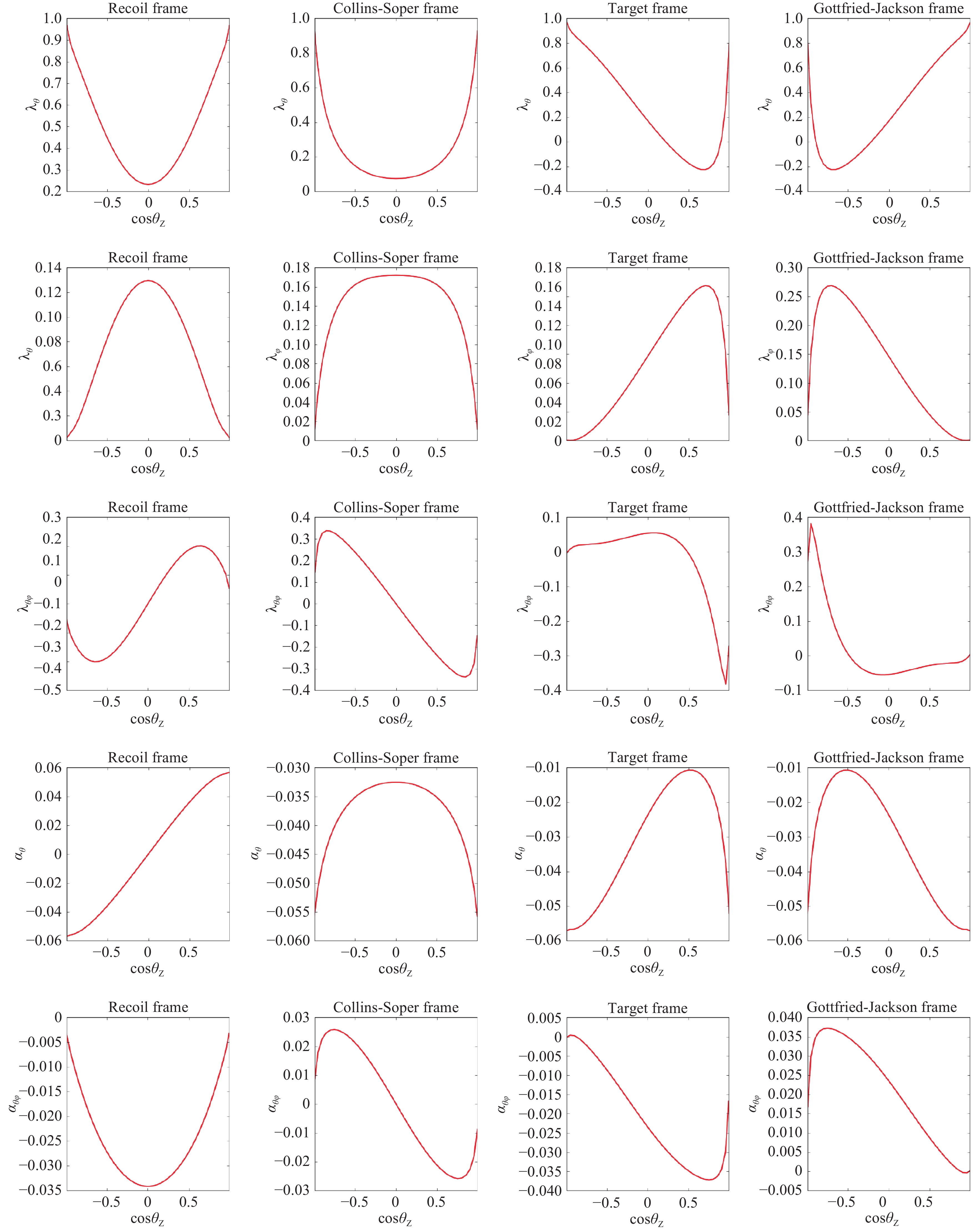Figure3. (color online) Angular distribution coefficients of the inclusive Z boson production dependence on cosθ_Z.

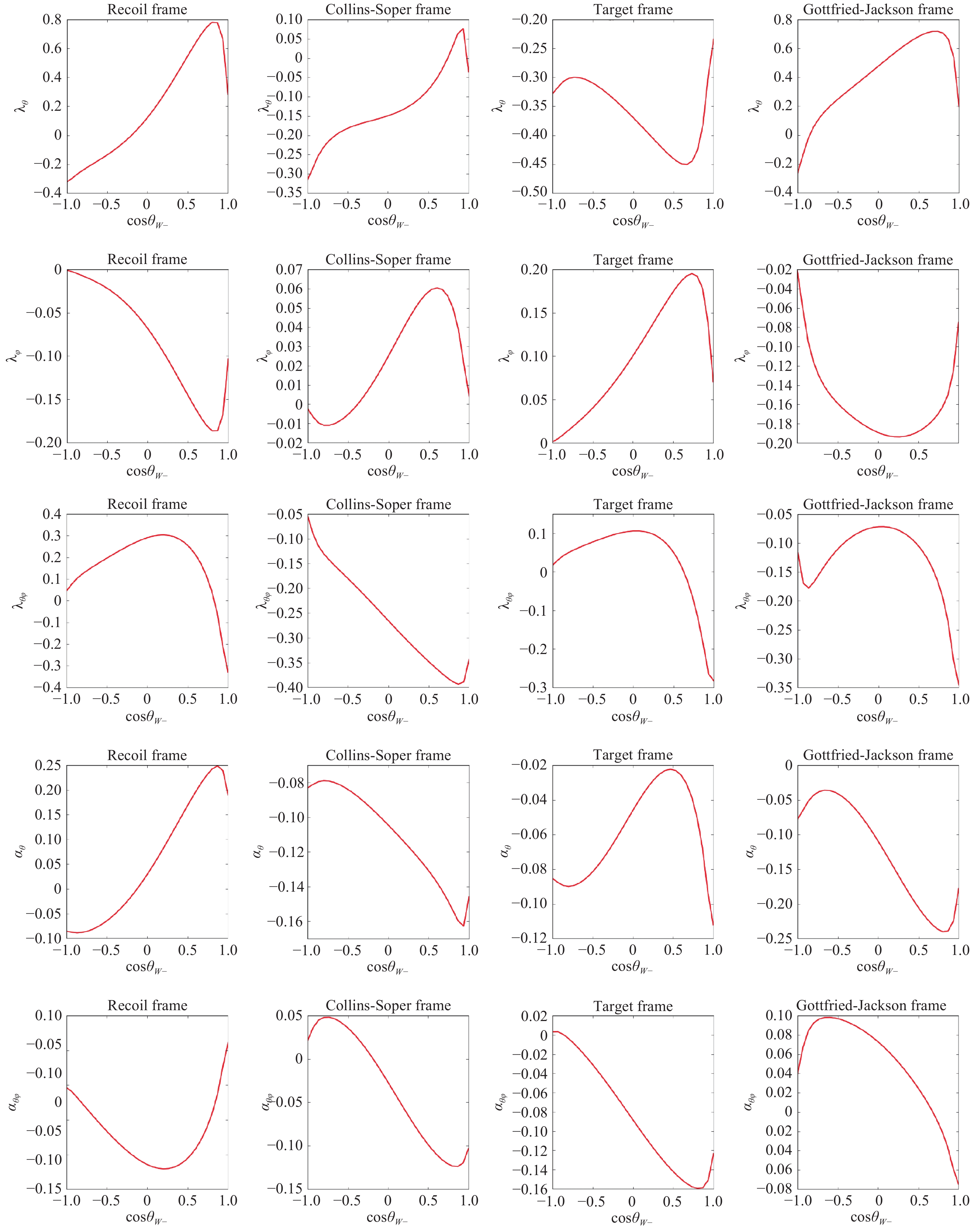Figure4. (color online) Angular distribution coefficients of the inclusive W^? boson production dependence on cosθ_W.

Then, in Fig. 4, the same plots for $ W^- $ productions are given. For more discussion about $ W^- $ production, refer to the process in the hadron collision [28]. At last, the angular distribution coefficients are calculated at different bins of $\mathrm{cos}\theta_Z$($\mathrm{cos}\theta_W$) in the Collins-Soper frame, as listed in the Table 4 and Table 5 .

cos$ \theta_Z $	$ \lambda_\theta $	$ \lambda_\varphi $	$ \lambda_{\theta \varphi} $	$ \alpha_\theta $	$ \alpha_{\theta\varphi} $
?1.0?0.99	0.996	0	0.015	?0.028	0
?0.99?0.94	0.843	0.017	0.196	?0.054	0.012
?0.94?0.9	0.723	0.024	0.228	?0.050	0.015
?0.9?0.7	0.480	0.086	0.291	?0.045	0.022
?0.7?0.45	0.335	0.110	0.223	?0.040	0.019
?0.45 ? 0	0.216	0.135	0.100	?0.036	0.009
0?0.45	0.216	0.135	?0.100	?0.036	?0.009
0.45?0.7	0.335	0.110	?0.223	?0.040	?0.019
0.7?0.9	0.480	0.086	?0.291	?0.045	?0.022
0.9?0.94	0.723	0.024	?0.228	?0.050	?0.015
0.94?0.99	0.843	0.017	0.196	?0.054	0.012
0.99?1.0	0.996	0	0.015	?0.028	0

Table4.Angular distribution coefficients for Z boson production at each bin in cos$ \theta_Z $ at C-S frame.

cos$ \theta_W $	$ \lambda_\theta $	$ \lambda_\varphi $	$ \lambda_{\theta \varphi} $	$ \alpha_\theta $	$ \alpha_{\theta\varphi} $
0?0.454	0.328	?0.105	0.295	0.652	?0.776
0.454?0.707	0.635	?0.160	0.209	1.288	?0.597
0.707?0.891	0.772	?0.185	0.019	1.598	?0.226
0.891?0.987	0.688	?0.171	?0.180	1.592	0.136
0.987?1	0.250	?0.098	?0.290	1.206	0.356

Table5.Angular distribution coefficients for $ W^- $ boson production at each bin in cos$ \theta_Z $ at C-S frame.

We present the detailed definitions of the theoretical calculation and experimental measurements on the lepton angular distribution coefficients of inclusive Z(W) boson production, necessary for the designed CEPC. The general expression of the cos$ \theta $ dependence for lepton angular distribution coefficients in the Z boson rest frame are represented by the production density matrix elements of $ e^++e^-\to Z +X $, and their range is given.
From the numerical results, it is clear that the event number estimated has the lepton pair estimated at the CEPC has the same order of magnitude as that of the ATLAS. The better accurate measurements are expected because there is less background. In comparison with the case at the hadron collider, the measurement for W is of a advantage because the momentum of the missing antineutrino from $ W^- $ decay can be obtained, and then, $ W^- $ is reconstructed. The two jets decay channels of Z(W) can also be measured with less background. The angular distribution coefficients of Z(W) boson production dependence of cos$ \theta_Z $ (cos$ \theta_W $) is calculated in four different polarization frames. Furthermore, the values of the angular distribution coefficients in different bins of cos$ \theta_Z $ are presented in the C-S frame. The calculation and results in this paper provide a method to precisely test the electroweak production mechanism or some effects from new physics in future measurements at the CEPC.
Further studies should be conducted that include Monte Carlo simulation with detector and background, the NLO electroweak correction for the production and Z(W) boson decay, NLO QCD correction to Z(W) boson decay, the correction to narrow width approximation, and initial-state-radiation effect. The NLO QCD correction to the angular distribution coefficients are less than 10% for the sum of all contributions in hadron collsions [4, 29]. In comparison with the hadron collision case, there is no NLO QCD correction at $ e^+e^- $ collider. The NLO electroweak correction is roughly estimated to be less than 1% because the coupling constant is smaller. This is outside the scope of this work and should be addressed in a future study.
We thank Dr. Bin Gong for the discussions.
2

-->

A.Appendix A: The relations of the density matrix elements

The production density matrix of the vector boson is written as$\, $

$\tag{A1}\sigma_{\lambda \lambda^\prime}= (M_\mu \epsilon^\mu_\lambda)(M_\nu \epsilon^\nu_\lambda)^\ast, $

where $ \epsilon_\lambda $ is the polarization of the vector boson and $ \lambda=+, 0, - $, which is defined by

$\tag{A2}\epsilon_0= \epsilon_z, \epsilon_\pm= \displaystyle\frac{1}{\sqrt{2}}(\mp\epsilon_x-i\epsilon_y), $

By the definition of Eq. (A1) and rewriting $ M_\mu $ as $ M_\mu=M_{1\mu}+iM_{2\mu} $ that $ M_{1\mu} $, and $ M_{2\mu} $ is real (for the situation when there is no weak interaction in $ M_\mu $, $ M_2=0 $) .

$\tag{A3}\begin{split}& \sigma_{+ +}= (M_\mu \epsilon^\mu_+)(-M_\nu^\ast \epsilon^\nu_-) = \frac{1}{2}[(M_{1\mu}M_{1\nu}+M_{2\mu}M_{2\nu})(\epsilon_x^\mu\epsilon_x^\nu+ \epsilon_y^\mu\epsilon_y^\nu) -(M_{2\mu}M_{1\nu}-M_{1\mu}M_{2\nu})(\epsilon_y^\mu\epsilon_x^\nu-\epsilon_x^\mu\epsilon_y^\nu)], \\& \sigma_{- -}= (M_\mu \epsilon^\mu_+)(-M_\nu^\ast \epsilon^\nu_-) = \frac{1}{2}[(M_{1\mu}M_{1\nu} +M_{2\mu}M_{2\nu})(\epsilon_x^\mu\epsilon_x^\nu+\epsilon_y^\mu\epsilon_y^\nu) + (M_{2\mu}M_{1\nu}-M_{1\mu}M_{2\nu})(\epsilon_y^\mu\epsilon_x^\nu-\epsilon_x^\mu\epsilon_y^\nu)], \\& \sigma_{+ -}= (M_\mu \epsilon^\mu_+)(-M_\nu^\ast \epsilon^\nu_+) = -\frac{1}{2}(M_{1\mu}M_{1\nu}+M_{2\mu}M_{2\nu})[(\epsilon_x^\mu\epsilon_x^\nu-\epsilon_y^\mu\epsilon_y^\nu)+i(\epsilon_x^\mu\epsilon_y^\nu+\epsilon_y^\mu\epsilon_x^\nu)], \\ & \sigma_{- +}= (M_\mu \epsilon^\mu_-)(-M_\nu^\ast \epsilon^\nu_-) = -\frac{1}{2}(M_{1\mu}M_{1\nu}+M_{2\mu}M_{2\nu})[(\epsilon_x^\mu\epsilon_x^\nu-\epsilon_y^\mu\epsilon_y^\nu)-i(\epsilon_x^\mu\epsilon_y^\nu+\epsilon_y^\mu\epsilon_x^\nu)], \\& \sigma_{0 +}= (M_\mu \epsilon^\mu_0)(-M_\nu^\ast \epsilon^\nu_-) = -\frac{1}{\sqrt{2}}\epsilon_z^\mu\{[(M_{1\mu}M_{1\nu}+M_{2\mu}M_{2\nu})\epsilon_x^\nu+ (M_{2\mu}M_{1\nu}-M_{1\mu}M_{2\nu})\epsilon_y^\nu] \\ & \qquad~ -i[(M_{1\mu}M_{1\nu}+M_{2\mu}M_{2\nu})\epsilon_y^\nu-(M_{2\mu}M_{1\nu}-M_{1\mu}M_{2\nu}) \epsilon_x^\nu]\}, \\& \sigma_{+ 0}= (M_\mu \epsilon^\mu_+)(M_\nu^\ast \epsilon^\nu_0) = -\frac{1}{\sqrt{2}}\epsilon_z^\mu\{[(M_{1\mu}M_{1\nu}+M_{2\mu}M_{2\nu})\epsilon_x^\nu+ (M_{2\mu}M_{1\nu}-M_{1\mu}M_{2\nu})\epsilon_y^\nu] \\ & \qquad~ + i[(M_{1\mu}M_{1\nu}+M_{2\mu}M_{2\nu})\epsilon_y^\nu-(M_{2\mu}M_{1\nu}-M_{1\mu}M_{2\nu}) \epsilon_x^\nu]\}, \\& \sigma_{0 -}= (M_\mu \epsilon^\mu_0)(-M_\nu^\ast \epsilon^\nu_+) = \frac{1}{\sqrt{2}}\epsilon_z^\mu\{[(M_{1\mu}M_{1\nu}+M_{2\mu}M_{2\nu})\epsilon_x^\nu-(M_{2\mu}M_{1\nu}-M_{1\mu}M_{2\nu})\epsilon_y^\nu] \\ & \qquad~ + i[(M_{1\mu}M_{1\nu}+M_{2\mu}M_{2\nu})\epsilon_y^\nu+(M_{2\mu}M_{1\nu}-M_{1\mu}M_{2\nu}) \epsilon_x^\nu]\}, \\ & \sigma_{- 0}= (M_\mu \epsilon^\mu_-)(M_\nu^\ast \epsilon^\nu_0) = \frac{1}{\sqrt{2}}\epsilon_z^\mu\{[(M_{1\mu}M_{1\nu}+M_{2\mu}M_{2\nu})\epsilon_x^\nu-(M_{2\mu}M_{1\nu}-M_{1\mu}M_{2\nu})\epsilon_y^\nu] \\ & \qquad~ - i[(M_{1\mu}M_{1\nu}+M_{2\mu}M_{2\nu})\epsilon_y^\nu+(M_{2\mu}M_{1\nu}-M_{1\mu}M_{2\nu}) \epsilon_x^\nu]\} .\end{split}$

From the above calculation, we see that $ \sigma_{+ +} $ is not equal to $ \sigma_{- -} $, unless the situation that $ M_\mu $ is real. Besides, we obtain the following relations,

$\tag{A4}\begin{split}\sigma_{+ -}=& (\sigma_{- +})^\ast, \\\sigma_{+0}=& (\sigma_{0+})^\ast, \\\sigma_{-0}=& (\sigma_{0 -})^\ast,\end{split}$

If $ M_\mu $ is real, from Eq. (A4) we could obtain the relations as

$\tag{A5}\begin{split}\sigma_{+ +}=& \sigma_{- -}, \\\sigma_{+ -}=& (\sigma_{- +})^\ast, \\\sigma_{+0}=& (\sigma_{0+})^\ast=-\sigma_{0-}=-(\sigma_{-0})^\ast, \end{split}$