Na-Na Ma ^1,
, Hai-Fei Zhang ^2,
, Xiao-Jun Bao ^3,
, Hong-Fei Zhang ^1,
, 1.School of Nuclear Science and Technology, Lanzhou University, Lanzhou 730000, China
2.Northwest Institute of Nuclear Technology, Xi'an 710024, China
3.Department of Physics, Collaborative Innovation Center for Quantum Effects, and Key Laboratory of Low Dimensional Quantum Structures and Quantum Control of Ministry of Education, Hunan Normal University, Changsha 410081, China
Received Date:2018-10-08
Accepted Date:2019-01-03
Available Online:2019-04-01
Abstract:Atomic Mass Evaluation (AME2016) has replenished the latest nuclear binding energy data. Other physical observables, such as the separated energies, decay energies, and the pairing gaps, were evaluated based on the new mass table. An improved Weizs?cker-Skyrme-type (WS-type) nuclear mass model with only 13 parameters was presented, including the correction from two combinatorial radial basis functions (RBFs), where shell and pairing effects are simultaneously dealt with using a Strutinsky-like method. The RBFs code had 2267 updated experimental binding energies as inputs, and their correspondent root-mean square (rms) deviations dropped to 149 keV. For the training of other mass models by RBFs correction, rms deviations are clustered between 100 keV to 200 keV. Compared with other experimental quantities, the rms deviations calculated within the improved WS-type model falls between 100 keV and 250 keV. We extrapolate the binding energies to 12435 nuclei, which covers the ranges $ 8\leqslant Z\leqslant128 $ and $ 8\leqslant N\leqslant251 $ in the framework of the WS-type model with RBFs correction. Simultaneously, the ground state deformations $ \beta_{2, \; 4, \; 6} $ and all parts in the WS-type mass formula are presented in this paper. Finally, we tabulated all calculated characteristics within the improved formula and linked them to https://github.com/lukeronger/NuclearData-LZU: nuclear binding energies, one-nucleon and two-nucleon separation energies ($ S_{\rm{n, \; p, \; 2n, \; 2p}} $), $ \alpha $ and $ \beta $-decay energies ($ Q_{\alpha} $ and $ Q_{\rm{\beta^-, \; \beta^+, \; EC}} $), and the pairing gap $ \Delta_{\rm{n}} $ and $ \Delta_{\rm{p}} $.

HTML

--> --> -->

The nucleus is regarded as a many-body system in which nucleons interact with each other in an intricate manner. The ground state binding energy of a nucleus is one of its basic characteristic properties and has long served [1-8] not only as a test system for various theoretical and experimental developments that aimed at the accurate determination in some burgeoning nuclear physics areas, such as super-heavy nuclei and exotic nuclei, but also as an indispensable tool in many other branches of physics, such as astrophysics [9, 10].
Other basic characteristics are essential means for a better understanding of the new branches of nuclear physics, such as nuclear structures [11-14], the compound-nucleus mechanism of nuclear reactions including nuclear fission and fusion [15]. For example, one-nucleon and two-nucleon separation energies are regarded as a direct way of testing shell closure [15, 16] and further for finding new candidates for magic numbers in super-heavy nuclei. Decay energies, contained $ \alpha $ [17-19] and $ \beta $-decay energy, cluster emission [20, 21], and spontaneous fission [22, 23] are necessary inputs for studying the stabilities of nuclei and the probabilities of synthesizing new nuclei. Neutron and proton odd-even staggering (OES) of nuclear binding energies may reflect the pairing correlation effects inside the nucleus [11, 12]. Theoretically, estimating the contribution of pairing effects in nuclei is extracted from the nuclear binding energies [24-45].
The limitation or lack of experimental technique in aforementioned studies led to many types of theoretical mass models, where other basic characteristics can be determined.
The nuclear binding energy for a nucleus is given by $B(Z, A)=[ZM_{\rm{H}}+NM_{\rm{n}}-M(Z, A)]c^2 $. After the developments of several decades [1–8, 16, 46–56], two kinds of typical mass models are continuously proposed: local mass models and global ones. Each has both advantages and shortcomings. In general, the rms deviations in local mass models [57-60] are smaller than in most global mass models. Global mass models, where many up-to-date physical effects are considered and simultaneously fitted by all known experimental data, show a more powerful extrapolation ability than local mass models. The relativistic mean-field (RMF) model [46, 47], Hartree-Fock-Bogoliubov [48–50], finite-range droplet model (FRDM) [16], Doflo-Zuker (DZ) [51, 52], Weizs?cker-Skyrme (WS) model along with a series of modified WS mass models [53–55], a mass formula performed by Bhagwat [61], and other nuclear mass formulae [62] are representatives of global mass models. All the rms deviations of these global mass models roughly range from 260 keV to 2000 keV.
Recently, we developed a new macroscopic-microscopic Weizs?cker-Skyrme-type mass model [56, 63, 64], now referred to as the WS-type model, in which the pairing energy dealt with the Bardeen-Cooper-Schrieffer (BCS) theory [24], and ultimately the shell and pairing effects were integrated into the Strutinsky method [65, 66]. With the help of the two combinatorial radial basis functions (RBFs) corrections [67] (inspired by the radial basis function approach [64, 68–71]), the WS-type mass formula is further improved. With the publication of the new mass table (AME2016), more unknown nuclei can be extrapolated within the improved mass model and the RBFs correction, where these updated experimental data serve as new inputs in the RBFs correction.
The remainder of this paper is organized as follows: A detailed description of the Weizs?cker-Skyrme-type mass model and the two combinatorial RBFs corrections are presented in Section 2. In Section 3, the experimental binding energies of 2267 known nuclei (green squares in Fig. 1) and the additional 136 nuclei (violet balls) are used as inputs to the WS-type model, and other mass formulae are trained by the RBFs corrections. Some systematic calculations for the known and the extrapolated 12435 nuclei (green open squares) are extracted from the improved WS-type mass model, including the ground state deformations $ \beta_{2, \; 4, \; 6} $, all ingredients of the WS-type model, nuclear binding energies, separation and decay energies, as well as pairing gap energies, and they are shown in Section 4. We have summarized the work in Section 5. Finally, all basic characteristics of 12435 nuclei are tabulated and linked to https://github.com/lukeronger/NuclearData-LZU.
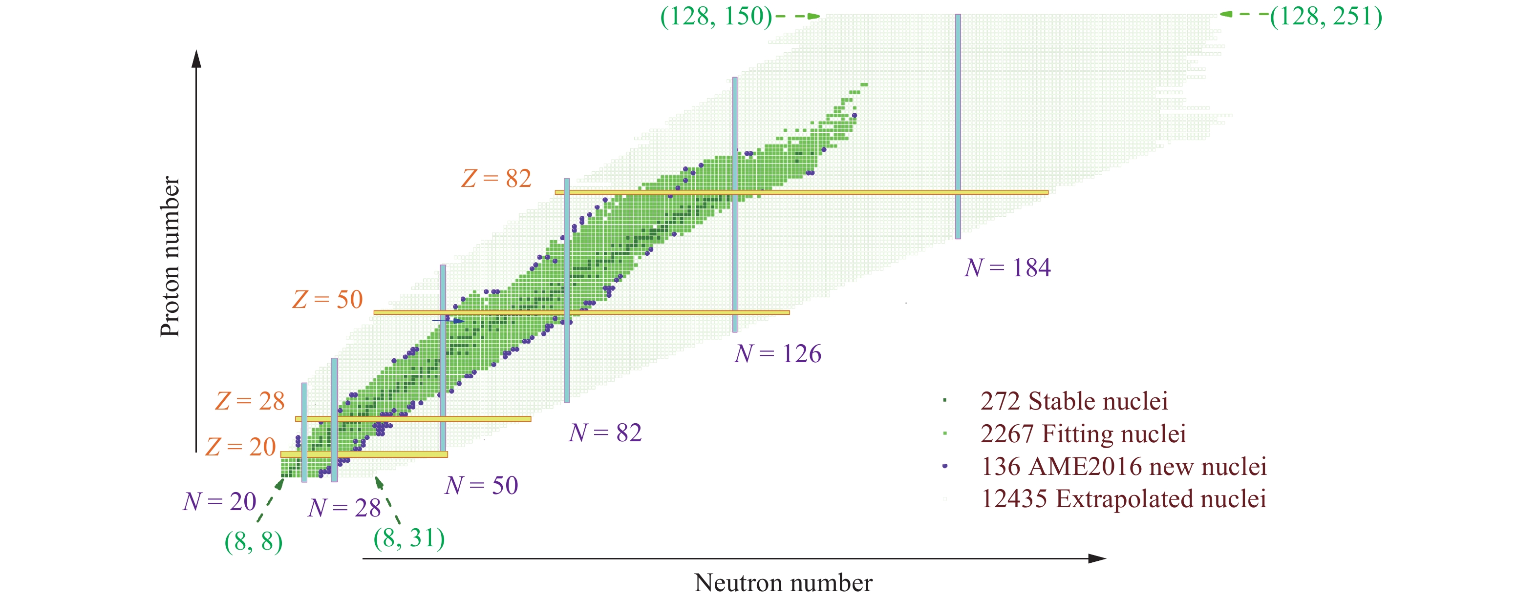Figure1. (color online) Nuclear landscape in this study, dark green squares denote 272 stable nuclei in AME2012; green squares represent 2267 nuclei selected to fit mass formula; additional 136 nuclei are labeled by violet balls, and the extrapolated 12435 nuclei are marked as open green squares.

Similar to most global nuclear mass models within the framework of the macroscopic-microscopic method, the original Weizs?cker-Skyrme-type (WS-type) mass model can be calculated as a sum of the macroscopic energy $ B_{{\rm{Mac}}} $, which was generally extracted from the liquid drop energy ($ B_{{\rm{LDM}}} $), and the microscopic energy $ B_{{\rm{Mic}}} $.
2

-->

2.1.Original WS-type mass model

The pairing correction in the Weizs?cker-Skyrme model [72] was $ E_{\rm{pair}}=a_{\rm{pair}}A^{-1/3}\delta_{{\rm np}} $, where the expression of $ \delta_{{\rm np}} $ depends on the values of the proton number Z and neutron number N, expressed as (here, $ I=(N-Z)/A $ [73])

$\delta_{{\rm np}}=\left\{ \begin{array}{*{20}{l}}2-|I|, \;\;\;& {N \; {\rm {and}} \; Z \; {\rm{even}}}\\|I|, \;\;\; &{N \;{\rm {and}} \; Z \; {\rm{odd}}}\\1-|I|, \;\;\; & {N \; {\rm{even}}, \; Z \; {\rm{odd}}, \; {\rm {and}} \; N>Z}\\1-|I|, \;\;\; &{{N \; {\rm{odd}}, \; Z \; {\rm{ even}}, \; {\rm {and}} \; N<Z}}\\1, \;\;\; &{{N \; {\rm{even}}, \; Z \; {\rm{ odd}}, \; {\rm {and}} \; N<Z}}\\1, \;\;\; &{{N \; {\rm{odd}}, \; Z \; {\rm{even}}, \; {\rm {and}} \; N>Z.}}\end{array} \right.$

The pairing correction was treated in a different manner in the WS-type model. We move the pairing term into the microscopic part $ B_{{\rm{Mic}}} $ and perform calculations using the standard BCS method. Shell and pairing effects are simultaneously evaluated by a procedure similar to the Strutinsky method (the detailed derivation of microscopic energy will be given later). For the WS-type mass model, the macroscopic part mainly contains volume, surface, Coulomb, and asymmetry terms. Therefore, the original WS-type mass formula [56] can be written as

$B(Z, A, \beta_k)= B_{{\rm{LDM}}}\prod_{k\geqslant 2}(1+b_k^2\beta_k^2) + B_{{\rm{Mic}}}(Z, A, \beta_k), $

(1)

where Z and A are the nuclear charge number and mass number, respectively. $ \beta_k $ is the deformation parameter, and $ b_k $ is explained in the following section.
3 -->

2.1.1.Macroscopic energy

Experimental results show that most nuclei displayed different deformations. Ref. [72] mentioned that, considering only axially deformed cases, the effects of nuclear deformation on the macroscopic energy exhibit a parabolic approximation, if the Skyrme energy-density function and the extended Thomas-Fermi approximation (ETF) were considered together. They had verified this parabolic approximation by calculating the binding energy ($ E_0 $) of spherical nuclei and the energies ($ E_{\beta_k} $) with different deformations via an integral over the Skyrme energy-density function under the ETF approximation. The curvature of the parabola for the different $ \beta_k $ deformation values can be approximately described as

$b_k = \left(\frac{k}{2}\right)g_1A^{1/3}+\left(\frac{k}{2}\right)^2g_2A^{-1/3}, \;\; k =2, 4, 6.$

(2)

where $ g_1 $ and $ g_2 $ are parameters fitted by the measured nuclear masses.
By considering the deformation effect (hence, our model is called Weizs?cker-Skyrme-type model), the extended macroscopic energy was expressed as

$\begin{split}B_{{\rm{Mac}}}(Z, A, b_k, \beta_k)=& [B_{\rm{Vol}}+B_{\rm{Surf}}+B_{\rm{Col}}+B_{\rm{Asy}}] \\& \displaystyle\prod_{k\geqslant 2}\left(1+b_k^2\beta_k^2\right), \end{split}$

(3)

where $ B_{\rm{Vol}} $ is the volume term, which provides a description of the saturation property of nuclear force, with $ I^2A $ being the asymmetry energy of the Bethe-Weizs?ker mass formula [74-77]. $ B_{\rm{Surf}} $ is the surface term considering the deficit of binding energy of nucleons at the surface, $ B_{\rm{Coul}} $ is the Coulomb term, which reproduced the Coulomb repulsion between protons [74], and $ B_{\rm{Asy}} $ is the asymmetry term, all of which are respectively given by

$\left\{ \begin{aligned}&B_{\rm{Vol}} =a_\nu(1+k_\nu I^2)A,\\ &B_{\rm{Surf}} =a_s(1+k_s I^2)A^{\frac{2}{3}},\\ &B_{\rm{Coul}} =a_c\displaystyle\frac{Z^2}{A^{\frac{1}{3}}}(1-0.76Z^{-2/3}),\\ &B_{\rm{Asy}} =c_1\displaystyle\frac{2-|I|}{2+|I|A}I^2A.\end{aligned} \right.$

Here, $ a_\nu, k_\nu, a_s, k_s, a_c, c_1 $ are model parameters, and including $ g_1 $ and $ g_2 $, there are eight adjustable parameters in the macroscopic part.
For consistency of parameters in the model between the macroscopic and microscopic parts, the isospin-dependent component of the macroscopic energy, including the asymmetrical part in volume term $ a_\nu k_\nu I^2 A $, surface term $ a_s k_s I^2 A^{2/3} $, asymmetry term $ c_1\displaystyle\frac{2-|I|}{2+|I|A} $, is approximately equal to the isospin-asymmetry part $ V_{s} $ of the Woods-Saxon potential depth in the microscopic part $ B_{{\rm{Mic}}} $, i.e.

$a_\nu k_\nu+a_s k_s/A^{1/3}+c_1\frac{(2-|I|)}{(2+|I|A)}\approx V_{s}.$

(4)

3 -->

2.1.2.Simultaneous calculation of the shell and pairing correction

To calculate the microscopic energy, one should diagonalize the Hamiltonian in axially deformed harmonic oscillator bases, where the code WSBETA [78] is applied. Single-particle levels and shell energy are calculated with the Strutinsky procedure.
An axially deformed Woods-Saxon potential depth is used in the calculation of the microscopic part. The central potential V takes the form of

$V=\frac{V_{{\rm{depth}}}}{1+{\rm{exp}}\left(\displaystyle\frac{r-R}{a}\right)}, $

(5)

where a is the diffuseness parameter of the central potential, and $ R=r_0A^{1/3} $ is the nuclear radius. $ V_{{\rm{depth}}} = V_0\pm V_s I $ denotes the depth of the central potential, with the addition for neutrons and the subtraction for protons. We assume that the isospin-asymmetry part of the potential depth $ V_s\approx a_\nu k_\nu+a_s k_s/A^{1/3}+c_1\displaystyle\frac{(2-|I|)}{(2+|I|A)} $ [see Eq. (4)]. $ V_0 $ is constant.
Whilst the isospin-orbit potential $ V_{{\rm{so}}} $ needs to be considered,

$V_{{\rm{so}}}=\lambda\left(\frac{\hbar}{2Mc}\right)^2\times \left\{\nabla \frac{V_{{\rm{depth}}}}{1+{\rm{exp}}\left(\displaystyle\frac{r-R}{a}\right)}\right\}\cdot(\vec\sigma\times \vec{p}), $

(6)

where combining the isospin-dependence, for proton $ \lambda = \lambda_0(1+Z/A) $, and for neutron $ \lambda = \lambda_0(1+N/A) $, both denote the strength of the spin-orbit potential.
The total single-particle Hamiltonian in this code was expressed as

$H = T + V+ V_{{\rm{so}}}.$

(7)

We evaluated the shell correction by using the standard Strutinsky approach, in which the Dirac generalized single-particle level density (SPLD) and the corresponding smoothed SPLD [79, 80] calculated with a convolution

$g(\varepsilon) =\sum\limits_{i=1}^Md_i\delta(\varepsilon-\varepsilon_i), $

(8)

$\bar g(\varepsilon) =\frac{1}{\gamma}\sum\limits_{i=1}^Md_iK\left(\frac{\varepsilon-\varepsilon_i}{\gamma}\right), $

(9)

where $ \varepsilon_i $ and $ d_i $ are the single-particle energy and its degeneracy, respectively. M denotes the number of single-particle levels. The function $ K(x) $ is a bell-shaped kernel and takes the Gauss-Hermit polynomials with the order p=6. $ \gamma=1.2\hbar\omega_0 $ is the smoothing width, and $ \hbar\omega_0=$$ 41A^{-1/3} $ MeV is the mean distance between the gross shells.
The standard BCS method is utilized to evaluate the pairing energy. The simplest seniority-type pairing force, the pairing interaction $ V_{{\rm{pair}}}=-Ga_i^\dagger a_{\bar i}^\dagger a_{\bar j}a_j $ is chosen, in which $ \bar k $ (for $ k=i, j $) denotes the label for the time-reversal partner of the k-th eigenstate of the single-particle Hamiltonian. Here, G is the pairing force strength. The pairing gap $ \Delta $ and the constraint on the expectation value of the number of particles were modified by the following two forms of SPLD, given by the standard gap equations

$\frac{2}{G}= \sum^M_{i=1}\frac{1}{\sqrt{(\epsilon_i-\lambda_{{\rm{BCS}}})^2+\Delta^2}}, $

(10)

$N= \sum^M_{i=1}\left[1-\frac{\epsilon_i-\lambda_{{\rm{BCS}}}}{\sqrt{(\epsilon_i-\lambda_{{\rm{BCS}}})^2+\Delta^2}}\right].$

(11)

The corresponding continuous expressions of the gap equations take form

$\frac{2}{G}=\frac{1}{2}\int^\infty_{-\infty}\frac{1}{\sqrt{(\epsilon-\bar\lambda_{{\rm{BCS}}})^2+\bar\Delta^2}}\bar g(\epsilon){\rm d}\epsilon, $

(12)

$N=\frac{1}{2}\int^\infty_{-\infty}\left[1-\frac{\epsilon-\bar\lambda_{{\rm{BCS}}}}{\sqrt{(\epsilon-\bar\lambda_{{\rm{BCS}}})^2+\bar\Delta^2}}\right]\bar g(\epsilon){\rm d}\epsilon.$

(13)

Here the pairing gap $ \Delta $ and the chemical potential $ \lambda_{{\rm{BCS}}} $ are determined by the two coupled equations for a given force strength G. $ \bar\lambda_{{\rm{BCS}}} $ denotes the Fermi level. The discrete BCS energy $ B_{\rm{BCS}} $ and the corresponding smoothed BCS energy $ \bar B_{\rm{BCS}} $ can be derived from Eq. (12) and Eq. (13), respectively

$\begin{array}{l}B_{\rm{BCS}}=\displaystyle\sum^M_{i=1}\left(1-\displaystyle\frac{\epsilon_i-\lambda_{\rm{BCS}}}{\sqrt{(\epsilon_i-\lambda_{\rm{BCS}})^2+\Delta^2}}\right)\epsilon_i-\displaystyle\frac{\Delta^2}{G}, \\\bar B_{\rm{BCS}}=\displaystyle\frac{1}{2}\displaystyle\int_{-\infty}^{\infty}\left[1-\displaystyle\frac{\epsilon_i-\bar\lambda_{\rm{BCS}}}{\sqrt{(\epsilon_i-\bar\lambda_{\rm{BCS}})^2+\bar\Delta^2}}\right]\epsilon\bar g(\epsilon){\rm d}\epsilon-\displaystyle\frac{\bar\Delta^2}{G}, \end{array}$

here $ \bar\Delta=\left(-12|\displaystyle\frac{N-Z}{A}|+7.5\right)/A^{1/3} $ in Ref. [81] is adopted. For simplicity, we set the radius and diffuseness of the single-particle potential of protons equal to those of neutrons.
The final average value $ B_{\rm p} $ of the pairing energy and the corresponding smoothed one $ \bar B_{\rm p} $ can be written as

$B_{\rm p} =B_{{\rm{BCS}}}-B_{\rm{s.p.}}, $

(14)

$\bar B_{\rm p} =\bar B_{{\rm{BCS}}}-\bar B_{\rm{s.p.}}.$

(15)

where $ B_{\rm{s.p.}} $ is the sum of all occupied single-particle level energies, $ \bar B_{\rm{s.p.}} $ is the smooth of $ B_{\rm{s.p.}} $, both extracted with the Strutinsky method [66, 67].
The pairing correction is defined as the difference between the pairing energy $ B_{\rm p} $ of the considered nucleus and that of an averaged value $ \bar B_{\rm p} $ for the same nucleus [82, 83]. The shell correction energy takes a similar form.

$B_{\rm{Pair}}= B_{\rm p}-\bar B_{\rm p}, $

(16)

$B_{\rm{Shell}}= B_{\rm{s.p.}}-\bar B_{\rm{s.p.}}.$

(17)

Substituting Eq. (15) into Eq. (16), together with Eq. (17), the microscopic correction energy $ B_{\rm{Mic}} $ derived from the Strutinsky approach and the BCS method is

$\begin{array}{l}B_{\rm{Mic}}= B_{\rm{Pair}}+B_{\rm{Shell}} = B_{\rm{BCS}}-\bar B_{\rm{BCS}}.\end{array}$

(18)

Further, the results of Ref. [53] indicate that considering the mirror nuclei constraint and the isospin-symmetry-breaking effect, the rms deviation of nuclear binding energy can be further reduced. Because an additional term $ |I|B_{\rm{shell}} $ can effectively reduce the shell correction deviation in pairs of mirror nuclei, we introduced a new parameter $ f_1 $, which is a scale factor of the microscopic energy [see Eq. (18)]. Thus the final microscopic energy takes the form of

$B_{\rm{Mic}}=f_1B_{\rm{Mic}}+|I|B'_{\rm{Shell}}.$

(19)

2 -->

2.2.Two combinatorial radial basis functions correction

The RBF approach [68, 69] as one of image reconstruction techniques has been adopted in the mass formula to improve the accuracy of nuclear binding energies [64, 70]. One would expect that the other physical observable could be improved at the same time. However, this fails to account for odd-even staggering (OES) of binding energies captured by nuclear mass, which is generally utilized to characterize the nuclear pairing correlation. One-nucleon separation energy also deteriorated. Two combinatorial radial basis function prescriptions (with the name of RBFs correction [65]) as a well-handled RBF approach assimilated the virtues of RBF approach and added the odd-even effects simultaneously. The RBFs approach has shown significant improvements with respect to the above-mentioned physical quantities of nuclei in Ref. [65].
First, the operation of the general RBF approach must be known. For a given nucleus, the reconstructed smooth function $ S(x) $ is

$S(x)=\sum\limits_{i=1}^{m}\omega_i\phi(||x-x_i||), $

(20)

where m is the number of data points to be fitted; $ x_i $ denotes the point from measurement, and $ \omega_i $ is the weight of the center $ x_i $. $ ||x -x_i|| $ is the Euclidean norm and the radial basis function $ \phi(r)=r $. Here, r denotes the distance between two nucleus $ (Z_i, N_i) $ and $ (Z_j, N_j) $

$r=\sqrt{(Z_i-Z_j)^2+(N_i-N_j)^2}.$

(21)

The weight $ \omega_i $ is obtained by solving the matrix equation

$\left(\begin{array}{c}\omega_1\\\omega_2\\\cdots\\\omega_m\end{array}\right)=\left(\begin{array}{cccc}\phi_{11} & \phi_{12} & \cdots & \phi_{1m}\\\phi_{21} & \phi_{22} & \cdots & \phi_{2m} \\\cdots & \cdots & \cdots & \cdots\\\phi_{m1} & \phi_{m2} & \cdots & \phi_{mm}\end{array}\right)^{-1}\left(\begin{array}{c}f_1\\f_2\\\cdots\\f_m\end{array}\right), $

(22)

with $ \phi_{ij}=\phi(||x_i -x_j||) \; (i, j=1, ..., m) $. $ f_i $ denotes the deviation between the experimental binding energy and the calculated one.
Inserting the weight $ \omega_i $ and the radial basis function $ \phi(||x-x_i||) $ into Eq. (20), the reconstructed smooth function $ S(Z, N) $ are obtained. Thus, the nuclear binding energy calculated with the RBF correction is the sum of the original calculated binding energy and $ S(Z, N) $.
As the first step, for a given nucleus, 2266 known binding energies of nuclei in the atomic mass evaluation of 2016 (AME2016) [6–8] are used to train the RBF approach. Thus, m = 2266 and $ f_i=B_{\rm{Expt}}(Z, N)-B_{\rm{Orig}}(Z, N) $ in Eq. (22), where $ B_{\rm{Orig}} $ denotes the binding energy calculated within the original WS-type model. The first revised binding energy of a nucleus is given by

$B_{\rm{RBF}}(Z_i, N_i)=B_{\rm{Orig}}(Z_i, N_i)+S_{\rm{Orig}}(Z_i, N_i).$

(23)

Here, we mark the first reconstructed smooth function as $ S_{\rm{Orig}} $.
In the second step, according to the odd-even property, 2267 nuclei are divided into four categories: even-even, even-odd, odd-even, odd-odd. For a given nucleus, the congeneric nuclei are employed to train the RBF correction again. This means that the value of m depends on the number of congeneric nuclei. Deviations $ f_i $ are also modified as $ f_i=B_{\rm{Expt}}(Z_i, N_i)-B_{\rm{RBF}}(Z_i, N_i) $. Thus, we obtain a new set of reconstructed smooth functions, labelled $ S_{\rm{oe}}(Z, N) $. The total contribution from the RBFs correction is

$S_{\rm{Total}}(Z, N)=S_{\rm{Orig}}(Z, N)+S_{\rm{oe}}(Z, N), $

(24)

The final nuclear binding energy for a nucleus can be written as

$B_{\rm{RBFs}}(Z, N)=B_{\rm{Orig}}(Z, N)+S_{\rm{Total}}(x).$

(25)

2 -->

2.3.Numerical details and model parameters

There are 13 adjustable parameters: 8 parameters ($ a_\nu $, $ k_\nu $, $ a_s $, $ k_s $, $ g_1 $, $ g_2 $, $ a_c $, $ c_1 $) in macroscopic part and 5 parameters ($ V_0 $, diffuseness parameter a, radius parameter $ r_0 $, the strength of the spin-orbit potential $ \lambda_0 $, scale factor $ f_1 $) in the microscopic part.
The first step is the selection of the experimental binding energies of the known nuclei. In our model, 2267 selected nuclei [green squares in Fig. 1] are used to fit the 13 model parameters. All selected nuclei satisfied two conditions: N and Z are larger than 7, and the standard deviation uncertainty on the mass is lower than or equal to 150 keV, as in Ref. [5].
The second step is inputting a set of deformation values for 2267 nuclei. By varying these 13 adjustable parameters and searching for the minimal deviation of the 2267 nuclear masses from experimental data by using a nonlinear least squares fitting procedure, these new 13 parameters are fixed to calculate the deformation of nuclei. Thereby, the first round is finished. The second round is the repetition of the operations in the first round. The new parameters and deformations are taken as new inputs in every repetitive operation, until the rms deviation becomes minimal.
The third step involves proceeding with the RBFs correction (here, taking the new atomic mass evaluation (AME2016) in Ref. [6] as inputs).

2

-->

3.1.Nuclear binding energy of improved WS-type model

In our model, the optimal rms deviation between the calculated nuclear binding energies and the experimental ones is 493 keV, and the average discrepancy is ?0.0108 MeV [56]. The corresponding parameters are listed in Table 1.

$ a_\nu $	$ k_\nu $	$ a_s $	$ k_s $	$ a_c $	$ c_1 $	$ g_1 $
15.4654	?1.8391	?17.1929	?2.0516	?0.7082	?28.2525	0.0093
$ g_2 $	$ V_0 $	$ r_0 $	$ a $	$ \lambda_0 $	$ f_1 $
?0.4015	?44.9430	1.3880	0.7765	27.8003	0.8557

Table1.Thirteen model parameters of Weizs?cker-Skyrme-type mass formula.

The rms deviations of the improved model with RBFs correction are reduced to 149 keV. The deviations between the experimental and calculated binding energies are plotted in Fig. 2(a) and (b), respectively. Some obvious differences appear along with the closed shell and the collectively-deformed region in Fig. 2(a). With the RBFs correction, almost all deviations in Fig. 2(b) tightly populate the area between 0.25 and –0.25 MeV and become smaller than the deviations in Fig. 2(a). Especially in the region near the neutron and /or proton magic numbers, significant improvements have been achieved. This indicates that the original WS-type model does not function optimally in these regions. Fig. 2(c) displays the reconstructed smooth function $ S_{\rm{Total}} $ in the nuclear chart. Here, $ S_{\rm{Total}} $ denotes the contribution from the RBFs correction. As we expected, the reconstructed smooth function shows the same behavior with the deviations in Fig. 2(a). Because $ S_{\rm{Total}} $ depends on the weight $ omega_i $ for a given nucleus, and $ omega_i $ is determined by the deviations $ f_i $ and the distance between two nuclei.
Figure2. (color online) Contour map of differences between experimental and calculated binding energies for 2267 nuclei as a function of neutron and proton number. Horizontal and vertical dot-dashed lines denote neutron and proton magic numbers. (b) As in (a), but for improved WS-type model with RBFs correction. (c) Total reconstructed smooth function $ S_{\rm{Total}} $.

Six isotopes, O, Ca, Fe, Ba, Au, U, are chosen as examples in Fig. 3 to show the behaviors of six terms along with the increasing neutron number N in mass formula: the volume term $ B_{\rm{Vol}} $, surface $ B_{\rm{Surf}} $, Coulomb $ B_{\rm{Coul}} $, asymmetric $ B_{\rm{Asy}} $ [see Eq. (4)], microscopic $ B_{\rm{Mic}} $ [see Eq. (19)], and the total reconstructed smooth function $ S_{\rm{Total}} $ [see Eq. (24)] of the total binding energy. The volume term $ B_{\rm{Vol}} $, surface term $ B_{\rm{Surf}} $, and Coulomb part $ B_{\rm{Coul}} $ per nucleon are three crucial ingredients for the total binding energy of a nucleus. Meanwhile, the contributions from the asymmetric part $ B_{\rm{Asy}} $, microscopic part $ B_{\rm{Mic}} $, and the total reconstructed smooth function $ S_{\rm{Total}} $ per nucleon are much smaller in comparison, especially for isotopes in the middle-heavy and heavy nuclear subregions, such as Fe, Ba, Au, and U. Combined with the corresponding macroscopic and microscopic parameters listed in Table 1, 13 parameters in the WS-type model are in accordance with the other theoretical mass model. Hence, six terms show the same behaviors with other theoretical models. In addition, the corresponding energy for six terms are reasonable. For example, the microscopic energy $ B_{\rm{Vol}} $ per mass number in Fig. 3 is between 10 MeV to 16 MeV for every isotopic chain. This is in accordance with the parameter $ a_v $ in Table 1, which yields 15.4654 MeV, i.e., roughly between 15 to 16 MeV. For the microscopic energy, it is generally common to amount to several MeV. An interesting phenomenon displayed in isotope Ba (Z = 56) is that $ B_{\rm{Coul}}/A\approx B_{\rm{Surf}}/A $ (where A is the mass number of a nucleus).
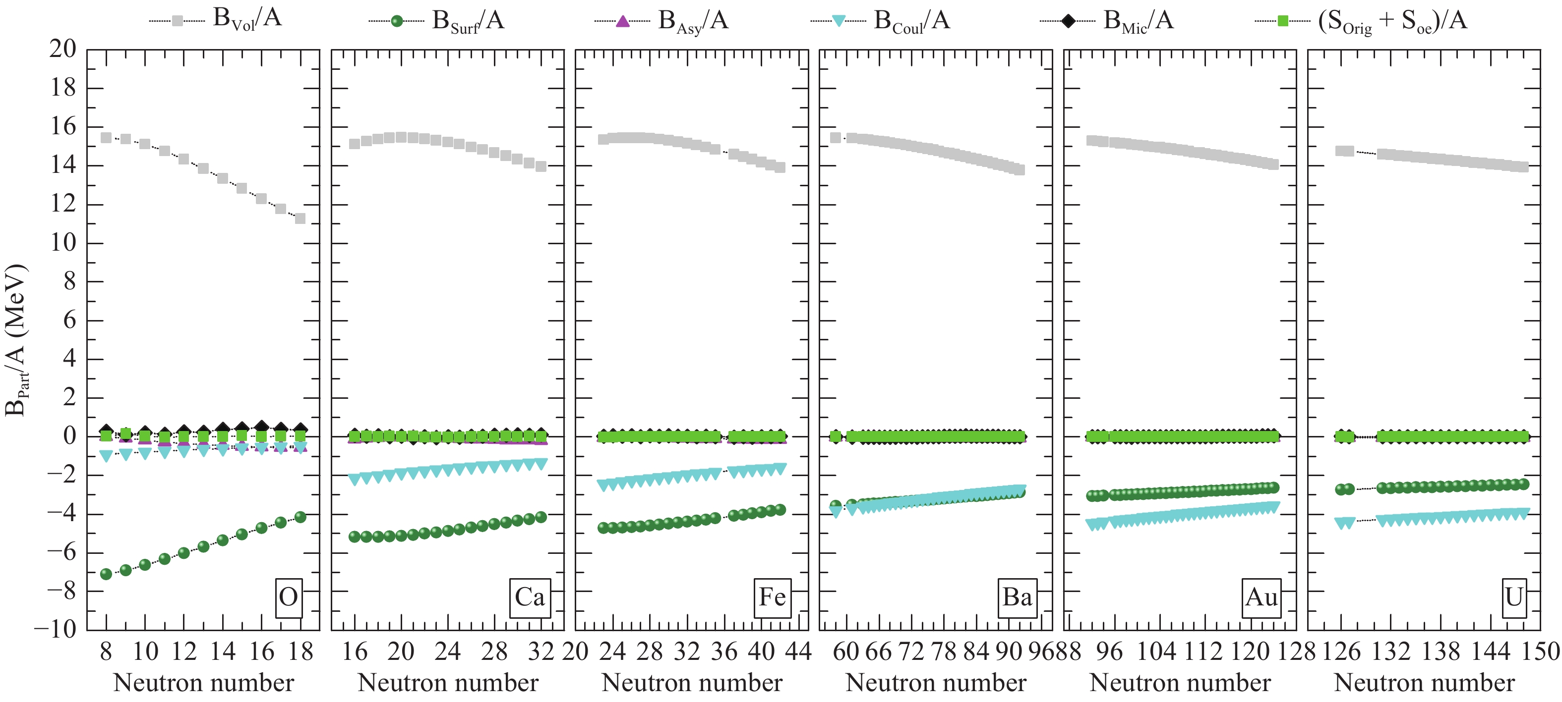Figure3. (color online) Six terms of total binding energy per nucleon in MeV. Light gray squares and dark green balls represent volume energy $ B_{\rm{Vol}} $ and surface term $ B_{\rm{Surf}} $, respectively. Magenta upward triangle and cyan downward triangle represent asymmetry term $ B_{\rm{Asy}} $ and Coulomb term $ B_{\rm{Coul}} $, respectively. Black diamonds correspond to microscopic term $ B_{\rm{Mic}} $ and green squares refer to the energies of total reconstructed smooth function $ S_{\rm{Total}}=S_{\rm{Orig}}+S_{\rm{oe}} $ per nucleon for six isotopes.

Furthermore, the 136 newly added nuclei in AME2016 [6] (compared with the atomic mass evaluation (AME2012) [5]) are used to investigate the effect of the RBFs correction. The spheres in Fig. 4 indicate the distributions of the additional 136 nuclei ($ 8\leqslant Z\leqslant 110 $). The discrepancies between experimental binding energies and the calculated ones within the original WS-type model are shown in the left panel in Fig. 4, with almost half of the 136 differences being larger than 0.5 MeV. These revised discrepancies ($ \Delta B=B_{\rm{Expt}}-B_{\rm{RBFs}} $) are calculated with the improved model in the right panel and are smaller than the results in the left panel, with most deviations clustered between ?0.2 and 0.2 MeV.
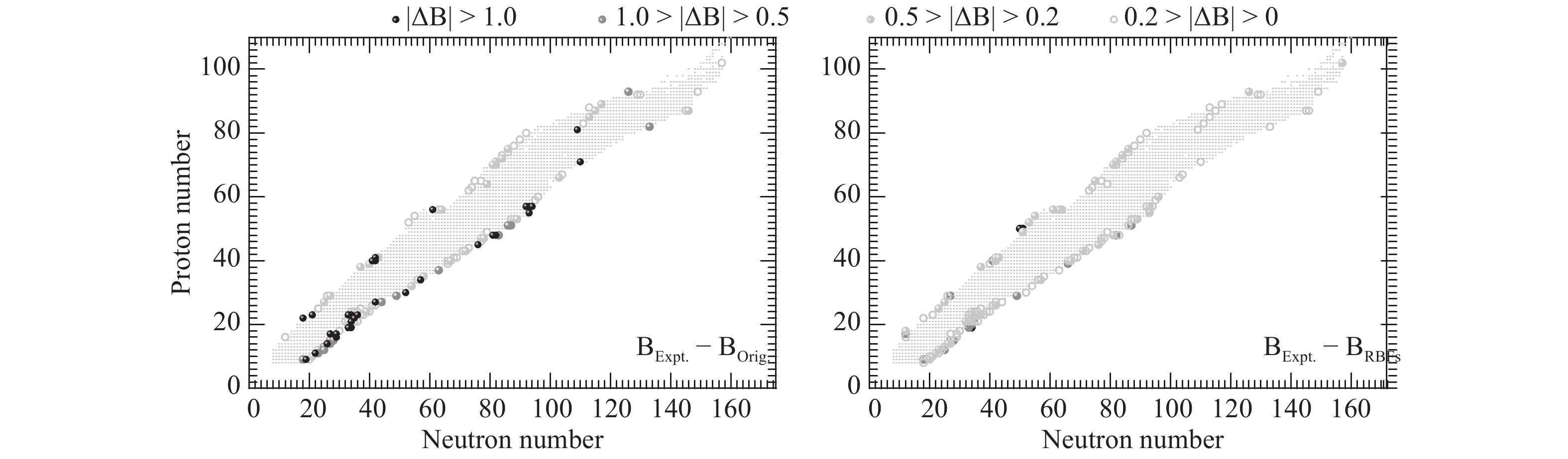Figure4. (color online) Two kinds of deviations between measured binding energies (in AME2016) and WS-type model predictions with/without the RBFs correction for 136 new added nuclei. Black balls denote the deviations of $ |\Delta B|>1 $ MeV. Gray and light gray balls and open balls represent the deviations of $ 0.5 < |\Delta B| < 1 $, $ 0.2 < |\Delta B| < 0.5 $, $ 0 < |\Delta B| < 0.2 $ MeV, respectively.

2 -->

3.2.Other nuclear mass formulae

With the incorporation of the RBFs correction, Fig. 5 gives insight into the dependence of the rms deviations on the sectionalized subregions for other mass models, i.e. WS-type, DZ31 [52], FRDM [16], WS4 [55], Bhagwat [61], and RMF [47]. Similar to the partitions in Ref. [56], the global region ($ Z, N\geqslant 8 $), light ($ 8\leqslant Z < 28 $), medium-I ($ 28 \leqslant Z < 50 $), medium-II ($ 50 \leqslant Z < 82 $), and heavy ($ Z\geqslant 82 $) are respectively labeled by G, L, M-I, M-II, and H.
Figure5. (color online) Two kinds of rms deviations calculated using original six models (blue stars) and improved models with RBFs correction (magenta balls) for five subregions, global (all nuclei with $ Z, N\ge 8$) (labeled by G), light ($ 8\leqslant Z < 28 $) (labeled by L), medium-I ($ 28\leqslant Z < 50 $) (labeled by M-I), medium-II ($ 50\leqslant Z < 82 $) (labeled by M-II), and heavy ($ Z\geqslant 82 $) (labeled by H). Rms of the global region is given in light cyan area.

Four main results are summarized in Fig. 5: (i) the WS4 model gives the best description without the RBFs correction (blue stars) compared to other models; (ii) all rms deviations of the six models with the RBFs correction (magenta balls) are reduced to 100–200 keV in the global region; (iii) these dependences show similar behaviors for the WS-type, DZ31, FRDM, WS4, and Bhagwat models with/without the RBFs approach. The RMF model shows different trends from the other five models; (iv) all of the deviations within the RBFs correction show similar trends in the six models.
There are additional 37 nuclei in the region where $ Z\geqslant $ 100, which fall into the heavy subregion (labeled by H) from AME2016. Detailed distributions of these nuclei are demonstrated in Fig. 6(a). Four subgraphs on the right-hand side show two kinds of discrepancies between experimental binding energies and the theoretical calculations with/without the RBFs correction for the above-mentioned six mass models. Fig. 6(b) and Fig. 6(c) show that (i) compared with calculations of the original six models [Fig. 6(b)], all the revised deviations [($ B_{\rm{Expt}}- $$B_{\rm{RBFs}} $) in Fig. 6(c))] are sharply reduced and fall into the region of $ -0.5 < (B_{\rm{Expt}}- $$B_{\rm{Cal}}) < 0.5 $ MeV; (ii) most of the differences of DZ31, FRDM, and RMF models are larger than the expected range shown by light magenta band in Fig. 6(b). This means that most of the binding energies calculated with the three above-mentioned theoretical models are larger than the experimental data. Fig. 6(b) provides therefore a good motivation for improvement in the heavy subregion for above models.
Figure6. (color online) Distributions of newly added 37 nuclei in H subregion ($ Z\geqslant82 $) in (a); two kinds of deviations for original and improved six mass models are shown in (b) and (c), respectively. Deviations of Bhagwat (blue open upward-pointing triangles), WS4 (green circles), WS-type (red open squares), DZ (dark green balls), FRDM (magenta stars), and RMF (cyan diamonds) models.

2

-->

4.1.The extrapolation of 12435 nuclei

After testing the availability of the RBFs correction by introducing it into the original mass models, the ultimate aim in this study is to calculate some basic characteristics of the 12435 nuclei ($ 8\leqslant Z\leqslant 128 $ and $8\leqslant $$ N\leqslant 251 $), as shown in Fig. 1 based on the improved WS-type model, including nuclear binding energies, one-nucleon and two-nucleon separation energy ($ S_{\rm{n}} $, $ S_{\rm{p}} $, $ S_{\rm{2n}} $, and $ S_{\rm{2p}} $), decay energy ($ Q_\alpha $, $ Q_{\beta^-} $, $ Q_{\beta^+} $, and $ Q_{\rm{EC}} $) as well as pairing gaps ($ \Delta_{\rm{n}} $ and $ \Delta_{\rm{p}} $).
In the WS-type model, the effects of nuclear deformation play a very important role in the description of nuclear binding energy. A deformed shape weakens the Coulomb energy and enhances the nuclear surface energy relative to a spherical one. In Fig. 7, we show the calculated ground state deformations of each nucleus with the WS-type model for all 12435 nuclei [see Eq. (2)]. Clearly, (i) the global amplitudes of the quadrupole deformation $ \beta_2 $ are larger than that of $ \beta_4 $, which in turn are larger than that of $ \beta_6 $; (ii) nearby the known traditional magic nuclei, $ \beta_{2, \; 4, \; 6}\approx0 $. This means that these nuclei are spherical or near spherical in shape; (iii) $ \beta_{4, \; 6} $ deformations in light nuclei (labeled by L) are not very obvious and increase with increasing neutron number; (iv) N = 184 is a candidate of the neutron magic number.
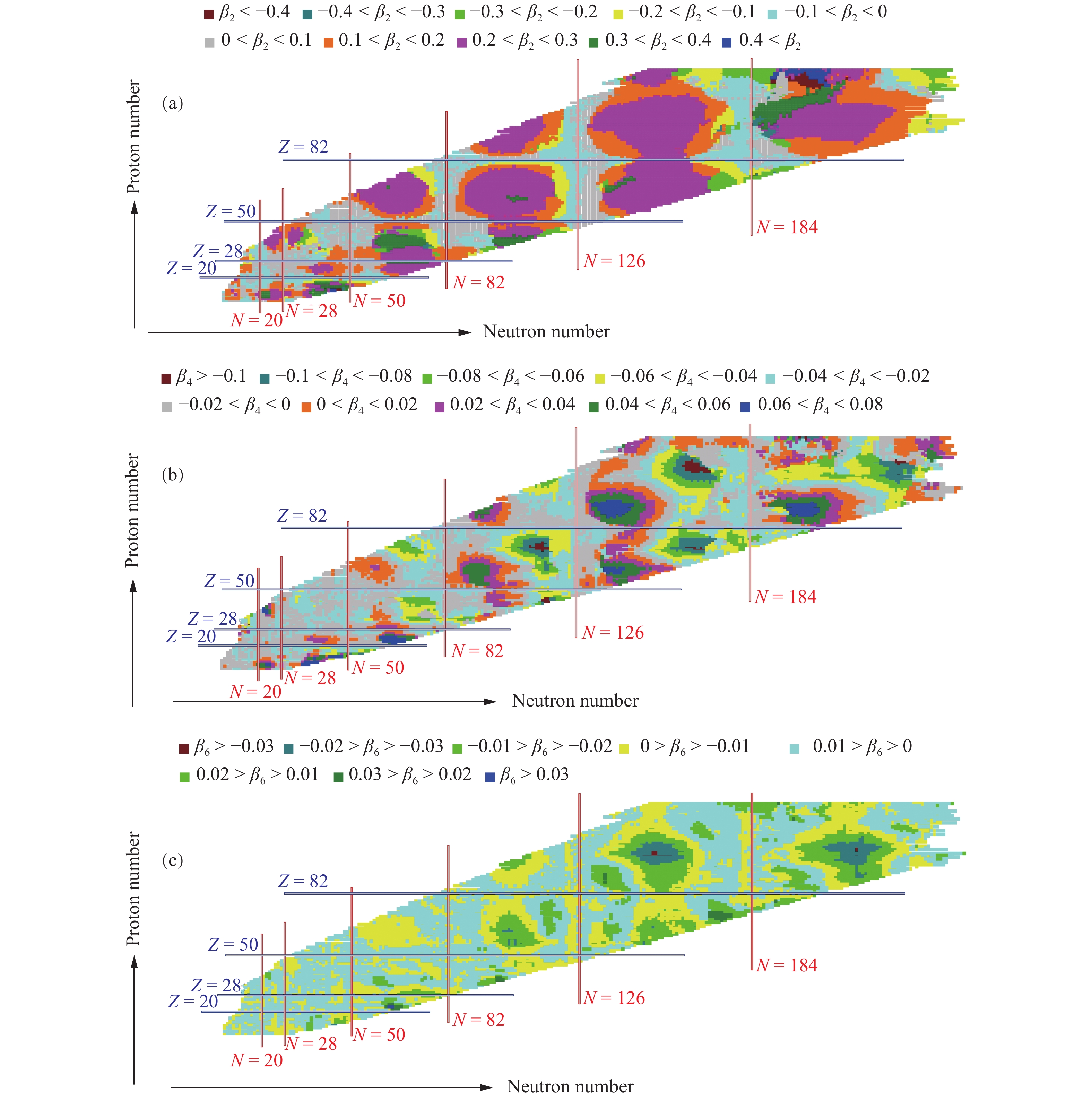Figure7. (color online) Three groups of deformations for 12435 nuclei, i.e. quadrupole deformations $ \beta_2 $and $ \beta_4 $, and $ \beta_6 $ as functions of neutron and proton numbers are shown in (a), (b), and (c), respectively. Traditional proton and neutron magic numbers are marked with blue and red lines, respectively.

For a given nucleus, six terms are included in the improved WS-type mass formula. They are the volume term, surface term, Coulomb term, asymmetry term and the microscopic term, as well as the total reconstructed smooth function. As in Fig. 3, Fig 8 displays the global behaviors of the aforementioned terms in a nuclear chart. It is observed that (i) $ B_{\rm{Vol}}/A $ (gray balls) and $ B_{\rm{Coul}}/A $ (dark green balls) are still dominant contributions to the total binding energy; (ii) $ B_{\rm{Surf}}/A $ (cyan balls) is large in the beginning and then decreases with increasing proton number; (iii) traditional magic numbers, Z = 28, 50, and 82 clearly appear in the microscopic energy $ B_{\rm{Mic}}/A $ (black balls); (iv) $ B_{\rm{Surf}}/A $, $ B_{\rm{Asy}}/A $ (magenta balls), $ B_{\rm{Mic}}/A $ and $ S_{\rm{total}}/A=(S_{\rm{Orig}}+S_{\rm{oe}})/A $ (green balls) and eventually get saturated with increasing proton numbers.
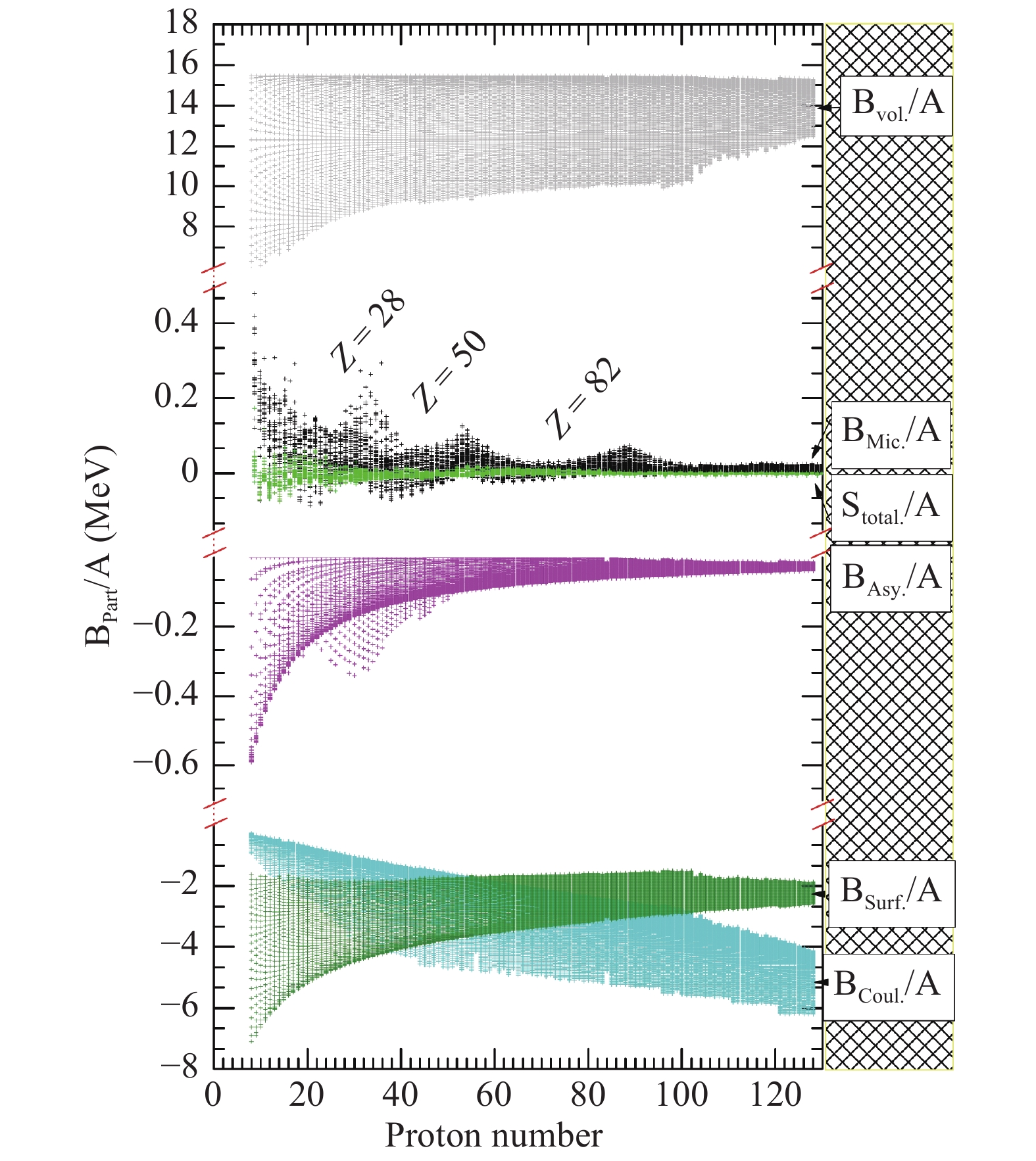Figure8. (color online) Six ingredients per nucleon of total binding energy for extrapolated 12435 nuclei are shown [same as Fig. 3]. Gray, cyan, dark green, black, and magenta balls, and green squares represent volume, surface, Coulomb, asymmetry, microscopy terms and the total reconstructed smooth function, respectively. Z = 28, 50, and 82 denote proton magic numbers.

2 -->

4.2.One-nucleon and two-nucleon separation energies

Generally, the statistical observable $ \sigma_{\rm{rms}} $ and the average values $ \cal{D} $ are introduced to estimate the reliability of theoretical models,

${\sigma _{{\rm{rms}}}} = \sqrt {\frac{1}{n}\sum\nolimits_{i = 1}^n | {B_{{\rm{Calc}}}} - {B_{{\rm{Expt}}}}{|^2}} ;$

(26)

${\cal{D}} = \frac{1}{n}\sum\nolimits_{i = 1}^n {[{B_{{\rm{Calc}}}} - {B_{{\rm{Expt}}}}]} , $

(27)

where $ B_{\rm{Calc}} $ and $ B_{\rm{Expt}} $ are the calculated and corresponding experimental binding energies, respectively.
One-nucleon and two-nucleon separation energies indicate how difficult it is to peel off one and two nucleons from the parent nucleus. Hence one- and two-neutron (proton) separation energies can be extracted from the nuclear binding energy by using the definition $ S_{\rm{n/2n}}(N, Z)=B(N, Z)-B(N-n/2n, Z) $$(S_{\rm{p/2p}}(N, Z)= B(N, Z)- $$B(N, Z-p/2p) $). The most striking application is to find some information about the shell structure. In particular, two nucleons separation energies are useful for finding new magic numbers in super-heavy and exotic nuclei [84, 85].
As mentioned before, when the general radial basis function is used to train the mass formula, the rms deviations of one-nucleon separation energy became larger than that of the original mass formula. Hence, we check the behavior of the one-neutron (proton) separation energy in the global nuclear chart.
Odd-even properties of nuclei are applied to divide 2267 nuclei into four categories, i.e. even (Z)-even (N), even-odd, odd-even, and odd-odd. The deviations between calculated one-neutron separation energies and experimental ones as functions of neutron and proton numbers are demonstrated in Fig. 9. Sub-graphs in the left column denote the deviations from the original WS-type mass formula. The right column depicts the WS-type with the RBFs correction. For even (Z)-even (N) nuclei, many deviations from the WS-type model are greater than 0.25 MeV, while the data for even-odd nuclei are less than ?0.25 MeV. By applying the RBF method, almost all deviations for four groups in the right column are smaller than that of data in the left column to a great extent. Furthermore, as we expected, the one-neutron separation energy for four groups in the left column exhibits the same behaviors and is in broad agreement with the experimental separation energy.
Figure9. (color online) Two types of deviations ($ S_{\rm n}^{\rm{Expt}}-S_{\rm n}^{\rm{Calc}} $) for even-even nuclei, even-odd, odd-even, and odd-odd nuclei: sub-graphs in left column—the results of original WS-type model, right column—original mass with RBFs correction. Horizontal and vertical dot lines denote neutron and proton magic numbers, respectively.

The results of the one-proton and one-neutron separation energies are same, and they are plotted in Fig. 10. In contrast to the deviations in the left column in Fig. 9, this time, the data in the odd (Z)-even (N) group are less than –0.25 MeV. After incorporating the RBFs correction, the deviations of four groups in the right column are sharply reduced and, simultaneously, almost populated the area between 0.25 and ?0.25 MeV.
Figure10. (color online) Same as caption of Fig. 11, but for one-proton separation energy.

Detailed rms deviations $ \sigma_{\rm{rms}} $ and $ \cal{D} $ of one-neutron (proton) separation energies for 2267 known nuclei are listed in Table 2. Here, the values of $ \sigma_{\rm{rms}} $ and $ \cal{D} $ for two-neutron (proton) separation energies are tabulated to check the improvement of the two combinatorial radial basis functions correction on the WS-type model. One can find that all rms deviations $ \sigma_{\rm{rms}} $ extracted from the improved WS-type model (the last row) are systematically smaller than those of the original WS-type model (the row above), and tightly cluster between 130 keV and 165 keV. Simultaneously, the average value of $ \cal{D} $ is sharply reduced. This indicates that the RBFs method is an effective tool to improve the one- and two-nucleon separation energies simultaneously.

models	$ S_{\rm{n}} $	$ S_{\rm{p}} $	$ S_{\rm{2n}} $	$ S_{\rm{2p}} $
	$ \sigma_{\rm{rms}} $ /keV
WS-type	360	503	444	520
WS-type + RBFs	139	145	162	153
models	$ S_{\rm{n}} $	$ S_{\rm{p}} $	$ S_{\rm{2n}} $	$ S_{\rm{2p}} $
	$ \cal{D} $ /keV
WS-type	?14.24	13.31	25.42	?22.65
WS-type + RBFs	1.18	?2.72	0.31	?1.23

Table2.Statistical observable $ \sigma_{\rm{rms}} $ and average values $ \cal{D} $ [see Eq. (26) and Eq. (27)] for four separation patterns, i.e. $ S_{\rm{n}} $, $ S_{\rm{p}} $, $ S_{\rm{2n}} $, and $ S_{\rm{2p}} $ obtained from original and improved WS-type model.

Exploring the extreme cases of the proton-to-neutron ratio in a nucleus, in which protons and neutrons are bound by strong nuclear and the Coulomb forces, is an important topic in nuclear physics. This is related to the limits of the nuclear landscape. Neutron and proton drip-lines denote the boundaries delimiting the existence of stable nuclei. For each isotopic (isotonic) chain, the nucleon (proton) drip line on the neutron (proton)-rich side is at the extreme of this ratio and no stable nuclei can exist. One- and two-nucleon separation energies provide a direct judgment for these limits, i.e. if both the one- and two-nucleon separation energies for a given nucleus are positive, this nucleus is stable.
Due to the powerful extrapolation ability of macroscopic-microscopic nuclear mass formulae, one can extrapolate nuclear mass for many known nuclei based on these theoretical mass models. Here, we extrapolate the nuclear binding energies of 12435 nuclei ( $ 8\leqslant Z\leqslant128 $ and $ 8\leqslant N\leqslant251 $, green open squares in Fig. 1), in the framework of the WS-type mass model with the RBFs correction and then calculate one- and two-nucleon separation energies by using these extrapolated binding energies. We tabulate all calculated separation energies and link them to https://github.com/lukeronger/NuclearData-LZU. One-nucleon separation energies, $ S_{\rm{n}} $ and $ S_{\rm{p}} $, are scaled by colors and plotted in Fig. 11. Two-neutron and two-proton separation energies of 12435 nuclei are demonstrated in the upper and lower parts in Fig. 12, respectively. We find that: (i) as physically expected, four types of separation energies show the remarkable jump in the traditional magic number regions, Z, N = 20, 28, 50, 82, and 126. In addition, N = 184 is a possible candidate of neutron magic numbers, and both are shown in Fig. 11 and Fig. 12. (ii) One-nucleon separation energy $ S_{\rm{n/p}} $ for each nucleus is roughly half of the value of $ S_{\rm{2n/2p}} $. (iii) One-nucleon separation energies show a remarkable nuclear zig-zag behavior because of the odd-even staggering (OES) of binding energies. (iv) The behavior of $ S_{\rm{n}} $ in the up panel in Fig. 11 is the same as two-neutron data $ S_{\rm{2n}} $ in Fig. 12. One- and two-neutron separation energies, $ S_{\rm{n}} $ and $ S_{\rm{2n}} $, both decrease with increasing neutron number for an isotopic chain, and finally both become negative.
Figure11. (color online) One-neutron and one-proton separation energies for 12435 nuclei, scaled by colors. Double lines denote traditional neutron and proton magic numbers. Dark green squares represent 272 stable nuclei.

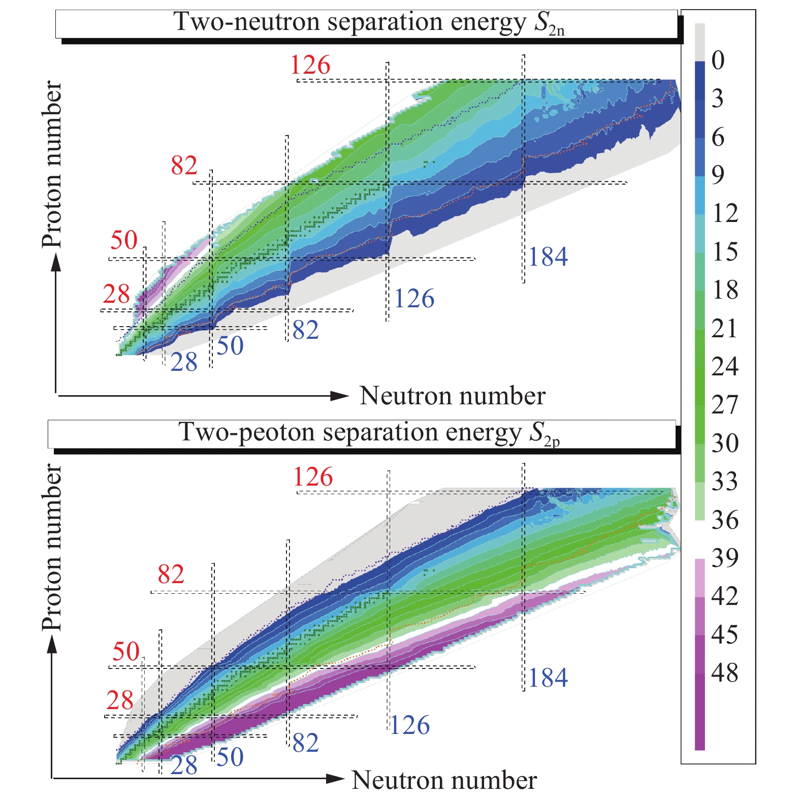Figure12. (color online) Consistently with Fig. 11, but for two-neutron (proton) separation energy. This time, contour plots are used.

With the behavior of the neutron separation energy, here we can further determine the neutron drip-line by using $ S_{\rm{n}}>0 $. As consistent behavior is presented in each isotonic chain, the proton drip-line can be extracted, i.e. $ S_{\rm{p}}>0 $. In Fig. 11 and Fig. 12, the violet dotted line represents the extracted proton drip-line, and the orange line represents the neutron drip-line under the framework of the improved WS-type model. All extrapolated figures also include plots of the 272 stable nuclei. Nuclei near or over the neutron and proton drip-lines are not stable. Hence, the existence probability of these nuclei is almost zero. In addition, the Coulomb interaction among protons leads to the experimentally known nuclei (green squares and violet balls in Fig. 1) that are near by the proton drip-line and far away from the neutron drip-line.
2 -->

4.3.alpha- and beta-decay energy

Between the neutron and proton drip-lines, nuclei have a reasonable probability to exist, and they preferably emit nucleons, such as alpha- and beta-particles, close to the valley of stability. The stability and radioactive decay of a nucleus are further related to the prediction of the 'island of stability' of superheavy nuclei (SHN) and their synthesis. Generally, several decay forms appear in many SHN, such as $ \alpha $-decay, $ \beta $-decay, electron capture, cluster emission, and spontaneous fission.
For heavy and superheavy nuclei, $ \alpha $-decay and spontaneous fission (SF) are two main processes that compete with each other. A mother nucleus emits an alpha-particle and then decays into a daughter nucleus, the process being referred to as alpha-decay. In general, alpha decay occurs only in some heavier nuclei. Alpha-decay energy $ Q_\alpha $ is an indispensable input for other theoretical models to study $ \alpha $-decay half-lives of nuclei. It is defined as

$Q_{\alpha}=B(\alpha)+B(Z-2, A-4)-B(Z, A), $

(28)

where $ B(\alpha)=28.296 $ MeV denotes the binding energy of the $ \alpha $ particle. $ B(Z, A) $ and $ B(Z-2, A-4) $ are the total binding energies of mother and daughter nuclei, respectively.
Another important decay form is beta-decay. There are three types of beta-decay: $ \beta^- $ decay, $ \beta^+ $decay, and the electron capture (EC). Unlike alpha decay, which is governed by the nuclear and Coulomb forces, beta-decay is a consequence of the weak force. The three types of beta decay energy, $ Q_{\beta^-} $, $ Q_{\beta^+} $, and $ Q_{EC} $, can be written as [86]

$Q_{\beta^-}=B(Z, A)- B(Z+1, A), $

(29)

$Q_{\beta^+}=B(Z, A)- B(Z-1, A), $

(30)

$Q_{\rm{EC}}=B(Z, A)- B(Z-1, A)-B_{\rm e}, $

(31)

where $ B_{\rm{e}} $ is the electron binding energy. $ B(Z, A) $ and $ B(Z-n, A) $ are the total binding energies of parent and daughter nuclei, respectively.
We extract the values of alpha- and beta-decay energies from the calculation of WS-type mass formulae with two combinatorial RBFs corrections. As in the one- and two-nucleon separation energies, we first tabulate the rms deviations $ \sigma_{\rm{rms}} $ and the average values of $ \cal{D} $ in Table 3 for alpha- and beta-decay energy by using Eqs. (26) and (27) to check the effect of the RBFs correction.

models	$ Q_\alpha $	$ Q_\beta^- $	$ Q_\beta^+ $	$ Q_{\rm{EC}} $
	$ \sigma_{\rm{rms}} $ /keV
WS-Type	464	504	503	504
WS-Type+RBFs	230	222	222	222
models	$ Q_\alpha $	$ Q_\beta^- $	$ Q_\beta^+ $	$ Q_{\rm{EC}} $
	$ \cal{D} $ /keV
WS-Type	13.78	20.35	?21.17	?20.59
WS-Type+RBFs	0.65	?1.56	1.58	1.55

Table3.Values of $ \sigma_{\rm{rms}} $ and $ \cal{D} $ [see Eq. (26) and Eq. (27)] for four decay energies: $ Q_\alpha $, $ Q_\beta^- $, $ Q_\beta^+ $, $ Q_{\rm{EC}} $.

Compared with the results from the original WS-type model, one can find the rms deviations of $ Q_\alpha $, $ Q_\beta^-$, $ Q_\beta^+ $, and $ Q_{\rm{EC}} $ evaluated by the WS-type with the RBFs method, marked as WS-type + RBFs, are sharply reduced from 500 keV to 200 keV. The values of $ \cal{D} $ also decrease. Furthermore, we calculate these four kinds of decay energies for the nuclei in the extrapolated nuclear landscape. Detailed data are listed at https://github.com/lukeronger/NuclearData-LZU. Fig. 13 demonstrates the alpha-decay values for nuclei $ 50\leqslant Z\leqslant 128 $ only, because alpha-decay typically occurs in some heavy and superheavy nuclei. There are 5657 nuclei that have positive decay energy, i.e. $ Q_\alpha > 0 $. The alpha-decay energy decreases with the neutron number for a given isotopic chain, while it increases with the proton number for a given isotonic chain. Nuclei near the neutron drip-line (orange dotted line) have negative values, which means that it is difficult for these nuclei to bring about alpha-decay. Along with stable nuclei (dark green squares) in Fig. 13, the $ Q_\alpha $ increases slowly, and most nuclei in this region have $ Q_\alpha < 4 $ MeV. In addition, alpha-decay values sharply change at the neutron and proton shell closure.
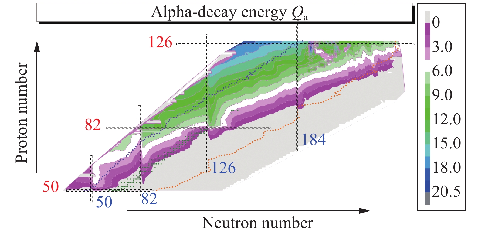Figure13. (color online) Contour plots of $ \alpha $-decay energies for four categories ($ Z\geqslant 50 $). Double dotted lines denote traditional neutron and proton magic numbers.

As the alpha-decay energy, $ \beta^- $-, $ \beta^+ $- and electron capture energy for the extrapolated nuclei are drawn in Fig. 14. For $ \beta^- $-decay, there are 7459 nuclei that have positive decay energy in first panel. We find that $ \beta^- $-decay generally occurs in neutron-rich nuclei, i.e. the region below the stable nuclei. Hence, these nuclei can convert a neutron to a proton, creating an electron and an electron-antineutrino, and thereby become more stable nuclei. We also find that $ Q_{\beta^-} $ increases along with increasing neutron number for an isotopic chain, while it decreases with the proton number for an isotonic chain. As expected, $ \beta^- $-decay occurs easily for nuclei approaching the neutron drip-line, and for nuclei close to the stable region, there is hardly any decay. The second and third panels show the $ \beta^+ $ and electron capture energy. There are 4793 nuclei, and 4523 nuclei have positive values for both decay modes, respectively. In contrast to the$ \beta^- $-decay, these two decay modes easily occur in proton-rich nuclei.
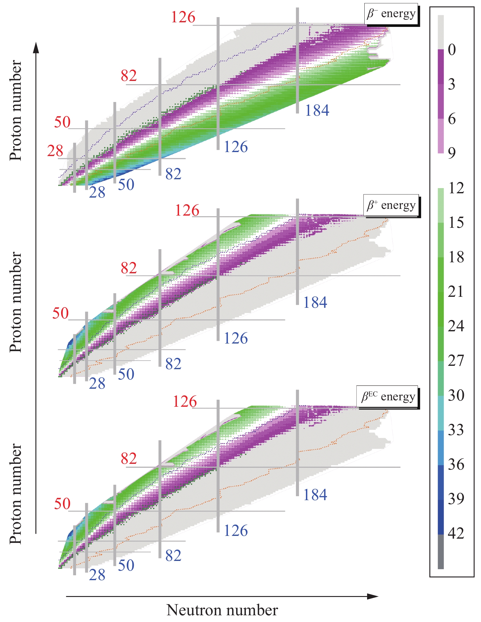Figure14. (color online)Contour plots of three kinds of $ \beta $-decay energies, i.e. $ \beta^- $-decay, $ \beta^+ $-decay and electron capture. Light gray lines denote traditional neutron and proton magic numbers.

2 -->

4.4.Neutron and proton pairing gap energy

In general, the phenomenological variation of the nuclear binding energy depends on the even and odd numbers of proton Z and neutron N. In other words, the systematic odd-even mass difference in nuclei, i.e. odd-even staggering (OES), was recognized previously and reflects the pairing correlation effect in nuclear structure. However, there is no direct way to measure the pairing effect. Theoretically, the five-point formulae are used to study the OES effect. For a given nuclear system with fixed N and Z, the expression of the neutron and proton pairing gaps can be written as [12, 87-89]

$\begin{split}\Delta_{\rm{n}}^{(5)}(N)\equiv &\frac{(-1)^N}{8}[B(N+2, Z)-4B(N+1, Z)\\&+6B(Z, N)-4B(N-1, Z)+B(Z, N-2)], \end{split}$

(32)

$\begin{split}\Delta_{\rm{p}}^{(5)}(Z)\equiv & \frac{(-1)^Z}{8}[B(N, Z+2)-4B(N, Z+1)\\&+6B(N, Z)-4B(Z-1, N)+B(Z-2, N)].\end{split}$

(33)

Here, we should note that the rms deviations of the neutron (proton) pairing gap from WS-type mass formula with the general RBF correction became worse than that of the original WS-type model in Ref. [65]. Here, we still need to verify if the two combinatorial RBFs corrections (RBF + RBFoe) can solve this problem.
Fig. 15 illustrates the differences in four categories between the experimental and theoretical pairing gap energy for 2267 nuclei, both calculated by five-point formulae. For even Z-even N and even Z-odd N groups in the upper panel of Fig. 15, the theoretical neutron pairing gap energy without the RBFs correction underestimates the real pairing gap values. Similarly, the calculated proton OES energies also underestimate the real values for even Z-even N and odd Z-even N groups in Fig. 15 (lower panel). By considering the RBFs correction, almost all deviations (red balls) populate the area between 0.4 and –0.4 MeV. Thus, we can make sure that the results improved by the RBFs correction yield a better agreement with experimental data.
Figure15. (color online) Two kinds of deviations for 2267 nuclei between experimental neutron pairing gap energies and theoretical data [original results (black open squares) and improved results (red balls)], both calculated using five-point formulae [see Eq. (33)] are shown. Same as neutron OES, deviations for proton OES calculated using Eq. (35) are shown in lower panel.

Intuitively, the rms deviations $ \sigma_{\rm{rms}} $ and average values $ \cal{D} $ of neutron OES and proton OES are displayed in Table 4, as in Table 2 and 3. The rms decreased to about 200 keV for both the neutron and proton pairing gaps with the RBFs correction. Together with the results from Fig. 15, we can make sure that the pairing energy in the framework of the WS-type mass formula with the RBFs correction reproduces the experimental data.

models	$ \Delta_{\rm{n}} ^5 $	$ \Delta_{\rm{p}}^5 $		$ \Delta_{\rm{n}}^5 $	$ \Delta_{\rm{p}}^5 $
	$ \sigma_{\rm{rms}} $ /keV			$ \cal{D} $ /keV
WS-Type	277	351		115.59	209.50
WS-Type+RBFs	169	150		8.25	2.60

Table4.As inTable 2, but for neutron and proton OES values: $ \Delta_{\rm{n}}^5 $ and $ \Delta_{\rm{p}}^5 $.

As for all aforementioned basic quantities, these two pairing gap energies are tabulated and attached in: https://github.com/lukeronger/NuclearData-LZU. Finally, neutron and proton pairing gap energies for the extrapolated 12435 nuclei are plotted in Fig. 16. Generally, neutron pairing gap energy decreases with increasing neutron number for an isotopic chain, while it increases with the proton number for an isotonic chain. Traditional neutron magic numbers are given in Fig. 16. Furthermore, N = 184 is a possible candidate of the neutron magic number. Meanwhile, the proton magic number at the proton shell closure is not so obvious. This is mainly because the pairing gap of $ \Delta_{\rm{n}} $ and $ \Delta_{\rm{p }} $ are expressed as $\bar{\Delta}=\left.\left(-12|\displaystyle\frac{N-Z}{A}|+7.5\right)\right/ $$ A^{1/3} $ in the WS-type mass model. This handling avoids additional parameters being added, while large deviations are introduced into some calculations with regards to the proton.
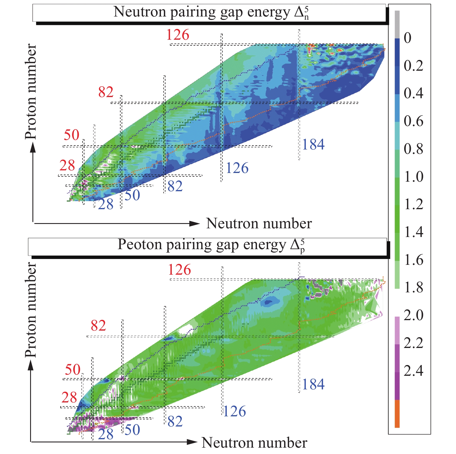Figure16. (color online) As in Fig. 15, but for neutron and proton pairing gaps of 12435 nuclei.

Two combinatorial RBFs corrections are introduced to modify the original WS-type model using new Atomic Mass Evaluation (AME2016). The root-mean square (rms) deviations for 2267 nuclei reduced to 149 keV within the improved WS-type model. Simultaneously, the deviations of separation energies, decay energies, and pairing gaps are sharply reduced to 100–200 keV. Other mass models, i.e. DZ31, FRDM, WS4, Bhagwat, and RMF are improved at the same time. It should be noted that the calculations for DZ31, FRDM, and RMF models give larger results than the experimental data in heavy subregion.
Furthermore, in the framework of the improved WS-type model, the following physical quantities for the extrapolated 12435 nuclei ($ 8\leqslant Z\leqslant128 $ and $ 8\leqslant N\leqslant251 $) are predicted and tabulated. These are two types of calculated binding energies with/without the RBFs correction, the total reconstructed smooth function $ S_{\rm{Total}} (S_{\rm{Orig}}+S_{\rm{oe}}) $, one- and two-nucleon separation energies (one-neutron $ S_{\rm{n}} $, one-proton $ S_{\rm{p}} $, two-neutrons $ S_{\rm{2n}} $, two nucleon $ S_{\rm{2p}} $), the alpha-decay energy $ Q_{\alpha} $, three types of $ \beta $-decay $ (Q_{\rm{\beta^-}}, Q_{\rm{\beta^+}}, Q_{\rm{EC}})] $, and the neutron (proton) pairing gap $ \Delta_{\rm{n}} $ ( $ \Delta_{\rm{p}} $).
We created a link to store the data package (see https://github.com/lukeronger/NuclearData-LZU). All physical quantities for the extrapolated 12435 nuclei in this data package are explained in Table 5. It can be downloaded by the git command or by contacting us via email (zhanghongfei@lzu.edu.cn).
We would like to thank Santosh Kumar Das and Baiyang Zhang for helpful discussions. N.M. is very thankful to Rong Wang for building this link.