Abdel Nasser Tawfik ^1,2,,
, Abdel Magied Diab ^3,,
, M.T. Hussein ^4,,
,

Corresponding author: Abdel Nasser Tawfik, atawfik@nu.edu.eg

Corresponding author: Abdel Magied Diab, a.diab@eng.mti.edu.eg

Corresponding author: M.T. Hussein, tarek@sci.cu.edu.eg

1.Nile University, Juhayna sq. of 26th-July-Corridor, 16453 Giza, Egypt
2.Frankfurt Institute for Advanced Studies, Ruth Moufang Str. 1, 60438 Frankfurt, Germany and World Laboratory for Cosmology And Particle Physics (WLCAPP), 11571 Cairo, Egypt
3.Egyptian Center for Theoretical Physics (ECTP), MTI University, 11571 Cairo, Egypt and World Laboratory for Cosmology And Particle Physics (WLCAPP), 11571 Cairo, Egypt
4.Physics Department, Faculty of Science, Cairo University, 12613 Giza, Egypt
Received Date:2018-03-25
Accepted Date:2018-12-05
Available Online:2019-03-01
Abstract:In characterizing the chiral phase-structure of pseudoscalar ($J^{pc}=0^{-+}$), scalar ($J^{pc}=0^{++}$), vector ($J^{pc}=1^{--}$) and axial-vector ($J^{pc}=1^{++}$t) meson states and their dependence on temperature, chemical potential, and magnetic field, we utilize the SU(3) Polyakov linear-sigma model (PLSM) in the mean-field approximation. We first determine the chiral (non)strange quark condensates, $\sigma_l$ and $\sigma_s$, and the corresponding deconfinement order parameters, $\phi$ and $\phi^*$, in thermal and dense (finite chemical potential) medium and finite magnetic field. The temperature and the chemical potential characteristics of nonet meson states normalized to the lowest bosonic Matsubara frequency are analyzed. We note that all normalized meson masses become temperature independent at different critical temperatures. We observe that the chiral and deconfinement phase transitions are shifted to lower quasicritical temperatures with increasing chemical potential and magnetic field. Thus, we conclude that the magnetic field seems to have almost the same effect as the chemical potential, especially on accelerating the phase transition, i.e. inverse magnetic catalysis. We also find that increasing the chemical potential enhances the mass degeneracy of the various meson masses, while increasing the magnetic field seems to reduce the critical chemical potential, at which the chiral phase transition takes place. Our mass spectrum calculations agree well with the recent PDG compilations and PNJL, lattice QCD calculations, and QMD/UrQMD simulations.

HTML

--> --> -->

Quantum Chromodynamics (QCD) predicts that the hadron-quark phase transition, where the hadronic matter goes through a partonic phase transition and generates a new-state-of-matter, colored quark-gluon plasma (QGP), takes place under extreme conditions of density (large chemical potential^①) and temperature. Accordingly, at high temperature and/or chemical potential, the confined hadrons are conjectured to dissolve into free colored quarks and gluons. Various heavy-ion experiments aim at characterizing the properties of this new-state-of-matter, for instance, STAR at the Relativistic Heavy-Ion Collider (RHIC) at BNL, ALICE at the Large Hadron Collider (LHC) at CERN, the future CBM at the Facility for Antiproton and Ion Research (FAIR) at GSI, and the future MPD at the Nuclotron based Ion Collider fAcility (NICA) at JINR.
The explicit chiral-symmetry breaking in QCD is assumed to contribute to the masses of the elementary particles [2-4]. In QCD-like models, which incorporate some features of QCD so that they are able to give an approximate picture of what the first-principle lattice QCD simulations can lead to, such as the Polyakov linear-sigma model (PLSM), or the Polyakov quark-meson (PQM) and the Polyakov Nambu-Jona Lasinio (PNJL) models, some properties of the QCD meson sectors can be studied numerically. In the present paper, we study the chiral phase-structure of sixteen meson states in a finite magnetic field and its dependence on temperature and chemical potential. To characterize the dependence of various meson masses for pseudoscalars ($J^{pc}=0^{-+}$), scalars ($J^{pc}=0^{++}$), vectors ($J^{pc}=1^{--}$) and axial-vectors ($J^{pc}=1^{++}$) on temperature, chemical potential and magnetic field, we utilize SU(3) PLSM in the mean-field approximation. The magnetic field is a significant ingredient to be taken into consideration, as it can be as high as $10^{19}\;$ Gauss in relativistic heavy-ion collisions. It is also conjectured that the deconfinement phase transition gives considerable contributions to the meson mass spectra. We shall discuss the conditions under which certain meson states dissolve into free colored quarks and gluons, and which temperature and chemical potential would be able to modify the chiral phase-structure of each of the nonet (sixteen) meson states.
It is not only the peripheral heavy-ion collisions that generate enormous magnetic fields, but also the central ones as well. Due to the opposite direction of relativistic charges (spectators), especially in non-central collisions and/or due to local momentum imbalance of the participants, a huge short lived magnetic field can be created. At SPS, RHIC and LHC energies, for instance, the mean values of such magnetic field have been estimated as ~0.1, ~1, and ~15$ m_{\pi}^2$, respectively [5-7], where $m_{\pi}^2 \simeq 10^{18}$ Gauss. It should be emphasized that such estimations were made with the Ultrarelativistic Quantum Molecular Dynamics model (UrQMD) for various impact parameters, i.e. different centralities.
It is noteworthy to highlight the remarkable influence of the Polyakov-loop potentials on scalar and pseudoscalar meson sectors. With the in (ex) clusion of the Polyakov-loop potentials in the LSM Lagrangian, the chiral phase-structure of the nonet meson states for finite temperatures has been evaluated [8]. The same study was carried out with(out) axial anomaly term [9, 10]. A systematic study of the thermal (temperature) and dense (chemical potential) influence on the chiral phase-structures of the nonet (sixteen) meson states with (out) axial anomaly term, and also with in (ex) clusion of the Polyakov-loop potentials, was published in [11]. For the sake of completeness, we recall that for finite chemical potential the SU(3) NJL model [12] and the SU(3) PNJL model [13-15] have been applied to characterize the nonet meson states as well.
The present work represents an extension of Ref. [11] to a finite magnetic field. We present a systematic study of the influence of the finite magnetic field, which is likely to be present in high-energy collisions, and the possible modifications on the chiral phase-structure of various (sixteen) mesonic states, including (pseudo) scalar and (axial) vector meson sectors, as function of temperature and chemical potential in the presence of a finite magnetic field. The temperature and chemical potential dependence of the chiral nonstrange and strange quark condensates, $\sigma_l$ and $\sigma_s$ , and the corresponding deconfinement order-parameters, $\phi$ and $\phi^*$, which determine the quark-hadron phase transitions in a finite magnetic field, shall be characterized for finite magnetic fields. We then investigate the various nonet meson states. Last but not least, we estimate how the normalization of these meson states relative to the lowest bosonic Matsubara frequency behaves with temperature, chemical potential and magnetic field. This allows to approximately determine the dissolving temperature and chemical potential for each meson state in a varying magnetic field.
An extensive comparison of our calculations of the meson nonets with the latest compilation of the Particle Data Group (PDG), lattice QCD calculations, and QMD/UrQMD simulations, shall be presented. It allows not only to characterize the meson spectra in thermal and dense medium, but also to describe their vacuum phenomenology in finite magnetic fields. We conclude that the results obtained are remarkably precise, especially for some light mesons, if these are extrapolated to vanishing temperatures.
The paper is organized as follows. We briefly describe the chiral LSM Lagrangian with three quark flavors in Section 2.1. We then give a short reminder of the PLSM model in the mean-field approximation in Section 2.2. In a vanishing or a finite magnetic field, the dependence of chiral nonstrange and strange quark condensates, and the corresponding deconfinement order-parameters characterizing the quark-hadron phase transition, on temperature and chemical potential, calculated form the SU(3) PLSM model, is presented in Section 3.1. The characterization of the magnetic catalysis is discussed as well. The chiral phase-structure of the various meson states in a finite magnetic field is outlined in Section 3.2. The temperature dependence of the chiral phase-structure of the sixteen meson states in a finite magnetic field is analyzed in Section 3.2.1. The chemical potential dependence is introduced in Section 3.2.2. Section 3.2.3 is devoted to the temperature dependence of these meson states normalized to the lowest Matsubara frequency. The conclusions are given in Section 4.

To study QCD thermodynamics and characterize the various nonet mesons for finite temperatures and chemical potentials, the linear-sigma model shall be utilized as an effective QCD-like model. In this section, we briefly describe the chiral phase-structure of the LSM Lagrangian with three quark flavors $N_f=3$, which can be established for fermionic and mesonic potentials. Concretely, the structure of this Lagrangian provides the tools to investigate the chiral phase-structure of nonet meson states. As we have done in a serious of previous publications, we treat SU(3) PLSM by means of the mean-field approximation, despite its well-know constrains. This approach enables to characterize the respective influence of finite magnetic field on the quark-hadron phase transition, in both thermal and dense medium. By a dense medium we mean, even if it might not be exactly equivalent with, a finite chemical potential. The intention is to examine the chiral phase-structure of the sixteen meson states. By doing this, we are able to compare their mass spectra with the experimental results, with the first-principle lattice QCD calculations, and with the corresponding estimations from other QCD-like models.
2

-->

2.1.Lagrangian of the linear-sigma model

As introduced in previous sections, LSM seems to give a remarkably good description of various meson states. With the increasing number of degrees of freedom, the quark flavors $N_f$, the number of meson states that can be generated increase as well. The full LSM Lagrangian in $U(N_f)$ with the color degrees of freedom $N_c$ is defined as ${\cal{L}}_{\rm chiral}={\cal{L}}_f+{\cal{L}}_m$, i.e. fermionic and mesonic sectors. In other words
● the first term represents quark (q) and antiquark fields ($\bar{q}$) [11],

$ {\cal{L}}_{f} =\bar{q} \left[i {\partial\!\!\!\!/}-g T_a \left(\sigma_a + i \gamma_5 \pi_a + \gamma _{\zeta} V_a ^{\zeta}+\gamma _{\zeta}\gamma _{5} A_a ^{\zeta} \right) \right] q, $

(1)

where g is the Yukawa coupling constant and $\zeta$ is an additional Lorentz index [16]
● the second term gives the mesonic Lagrangian, which consists of the various contributions of the nonet states, interactions and possible anomalies

$ \begin{aligned} {\cal{L}}_{m}&=&{\cal{L}}_{\rm SP}+ {\cal{L}}_{\rm VA}+ {\cal {L}}_{\rm Int}+ {\cal{L}}_{U(1)_A}, \end{aligned} $

(2)

where ${\cal{L}}_{\rm SP}$ stands for scalar ($J^{pc}=0^{++}$) and pseudoscalar ($J^{pc}=0^{-+}$), while ${\cal{L}}_{\rm AV}$ represent vector ($J^{pc}=1^{--}$) and axial-vector ($J^{pc}=1^{++}$) mesons. ${\cal{L}}_{\rm Int}$ represents interactions that take place in the system of interest. The last term is called an anomaly term $U(1)_A$. For more details about the mesonic Lagrangian, interested readers are kindly advised to consult Refs. [11, 17-24]. Further details about $U(N_f)_r \times U(N_f)_{\ell}$ can be obtained from [17-24]

$ \begin{split} {\cal{L}}_{\rm SP}=& {\rm{Tr}}\left[(D^{\mu}\Phi)^{\dagger} (D^{\mu}\Phi)-m^2 \Phi^{\dagger} \Phi\right]-\lambda_1 [{\rm{Tr}}(\Phi^{\dagger} \Phi)]^2 \\&-\lambda_2 {\rm{Tr}}(\Phi^{\dagger} \Phi)^2 + {\rm{Tr}}[H(\Phi+\Phi^{\dagger})], \end{split} $

(3)

$ \begin{split} {\cal{L}}_{\rm AV}=&-\frac{1}{4}\mathop{{\rm{Tr}}}\left(L_{\mu\nu}^{2}+R_{\mu\nu}^{2} \right)+\mathop{{\rm{Tr}}}\left[\left( \frac{m_{1}^{2}}{2}+\Delta\right) \left(L_{\mu}^{2}+R_{\mu}^{2}\right)\right] +i \frac{g_{2}}{2} (\mathop{{\rm{Tr}}}\{L_{\mu\nu}[L^{\mu}, L^{\nu}]\}+\mathop{{\rm{Tr}}}\{R_{\mu\nu}[R^{\mu}, R^{\nu}]\}){}+ g_{3}[\mathop{{\rm{Tr}}}(L_{\mu}L_{\nu}L^{\mu}L^{\nu} )\\ &+\mathop{{\rm{Tr}}}(R_{\mu}R_{\nu}R^{\mu}R^{\nu})]+g_{4} [\mathop{{\rm{Tr}}}\left( L_{\mu}L^{\mu}L_{\nu}L^{\nu}\right) +\mathop{{\rm{Tr}}}\left( R_{\mu}R^{\mu}R_{\nu}R^{\nu}\right) ]{} +g_{5}\mathop{{\rm{Tr}}}\left( L_{\mu}L^{\mu}\right) \mathop{{\rm{Tr}}}\left( R_{\nu}R^{\nu}\right) +g_{6} [\mathop{{\rm{Tr}}}(L_{\mu}L^{\mu}) \mathop{{\rm{Tr}}}(L_{\nu}L^{\nu })\\&+\mathop{{\rm{Tr}}}(R_{\mu}R^{\mu}) \mathop{{\rm{Tr}}}(R_{\nu}R^{\nu })], \end{split} $

(4)

$ {\cal{L}}_{\rm Int}=\frac{h_{1}}{2}\mathop{{\rm{Tr}}}(\Phi^{\dagger}\Phi )\mathop{{\rm{Tr}}}(L_{\mu}^{2}+R_{\mu}^{2})+h_{2} \mathop{{\rm{Tr}}}[\vert L_{\mu}\Phi \vert ^{2}+\vert \Phi R_{\mu} \vert ^{2}]+2h_{3} \mathop{{\rm{Tr}}}(L_{\mu}\Phi R^{\mu}\Phi^{\dagger}), $

(5)

$ {\cal{L}}_{U(1)_A}=c[{\rm{Det}}(\Phi)+{\rm{Det}}(\Phi^{\dagger})]+c_0 [{\rm{Det}}(\Phi)-{\rm{Det}}(\Phi^{\dagger})]^2 +c_1 [{\rm{Det}}(\Phi)+{\rm{Det}}(\Phi^{\dagger})] {\rm{Tr}} [\Phi \Phi^{\dagger}]. $

(6)

The complex matrices for scalar $\sigma_{a}$, i.e. $J^{PC}=0^{++}$, pseudoscalar $\pi _{a}$, i.e. $J^{PC}=0^{-+}$, vector $V_{a}^{\mu}$, i.e. $J^{PC}=1^{--}$ and axial-vector $A_{a}^{\mu}$, i.e. $J^{PC}=1^{++}$ meson states can be constructed as

$ \begin{split} \Phi =& \sum_{a=0}^{N_{f}^{2} -1} T_{a}(\sigma _{a}+ i \pi _{a}), \\ L^{\mu} = &\sum_{a=0} ^{N_{f}^{2} -1} T_{a} (V_{a}^{\mu}+A_{a}^{\mu}), \\ R^{\mu} =& \sum_{a=0}^{N_{f}^{2} -1} T_{a} (V_{a}^{\mu}-A_{a}^{\mu}). \end{split} $

(7)

The various generators are defined according to $N_f$. It is obvious that the covariant derivative, $D^\mu \Phi = \partial^\mu \Phi-$ $ i g_1 (L^\mu \Phi - \Phi R^\mu)$, is to be associated with the degrees of freedom for (pseudo-)scalar and (axial-)vector and couples them through $g_1$, the coupling constant. For instance, for $N_f=3$, the unitary matrices for ${SU}(3)_r \times $ $ {SU}(3)_{\ell}$ can be obtained from Ref. [11], while $T_{a}$, the generators of ${U}(3)$ , can be expressed as $T_{a}=\hat{\lambda}_{a}/2$, with $a=0\dots 8$ , and $\hat{\lambda}_{a}$ are the Gell-Mann matrices.
Different PLSM parameters have been fixed in previous studies [8, 25]. It should be noted that these two models are inconsistent and so is any parameterization based on them. The problem was solved in Ref. [4], where the authors introduced $C_1$ combining various parameters, $C_1=m_0^2+\lambda_1\left(\sigma_l^2+\sigma_s^2\right)$. While $C_1$ can only be estimated through parametrization, its individual parameters can not. While both $m_0^2$ and $\lambda_1$ were taken from Ref. [8], the remaining ones have been determined (see Table 3 in Ref. [25]).
2 -->

2.2.Polyakov linear-sigma model in the mean-field approximation

The LSM Lagrangian with $N_f=3$, which are coupled to $N_c=3$ , can be written as ${\cal{L}}={\cal{L}}_{\rm chiral}- {\cal{U}}(\phi, \phi^*, T)$. The potential ${\cal{U}}(\phi, \phi^{*}, T)$ should be adjusted from recent lattice QCD simulations. Accordingly, various LSM parameters can be determined. It should be noted that this Lagrangian has a $Z(3)$ center symmetry [26-29]. Through the thermal expectation values of the color traced Wilson-loop in the temporal direction, the dynamics of color charges and gluons can be taken into consideration

$ \begin{aligned} \phi = \langle{\rm{Tr}}_c {\cal{P}}\rangle/N_c, && \phi^* = \langle{\rm{Tr}}_c {\cal{P}}^{\dagger}\rangle/N_c. \end{aligned} $

(8)

The Polyakov-loop potential ${\cal{U}}(\phi, \phi^*, T)$ can be introduced in the pure gauge limit as the temperature and density dependent quantity. There are various proposals how to do so.
In previous works, we have implemented the polynomial potential [11, 30-32]. In the present work, we introduce calculations based on an alternatively-improved extension to $\phi$ and $\phi^{*}$ [27, 29, 33], the logarithmic potential,

$ \begin{split} \frac{{\cal{U}}_{\rm{Log}}(\phi, \phi^*, T)}{T^4} =& \frac{-a(T)}{2} \phi^* \phi \\&+ b(T) \ln{\left[1-6 \phi^* \phi + 4 ( \phi^{*3} + \phi^3)-3 ( \phi^* \phi)^2 \right]}. \end{split} $

(9)

where $T_0$ is the critical temperature for the deconfinement phase-transition in the pure-gauge sector,

$ \begin{aligned} a(T) = a_0 + a_1 \left(T_0/T\right) + a_2 \left(T_0/T\right)^2 \;{\rm{and}}\; b(T) = b_3 \left(T_0/T\right)^3, \end{aligned} $

(10)

The remaining parameters $a_0$, $a_1$, $a_2$, and $b_3$ can be determined by comparison with lattice QCD simulations. These are listed in Table 2 in Ref. [34].
In thermal equilibrium, the mean-field approximation of the Polyakov linear-sigma model can be implemented in the grand-canonical partition function ($\cal{Z}$) for finite temperature (T) and finite chemical potential ($\mu_f$). Here, the subscript f refers to the quark flavors. For finite volume (V), the free energy reads $\cal{F}=-T \cdot \log [\cal{Z}]/V$. For instance, for SU(3) PLSM,

$ {\cal{F}} = U(\sigma_l, \sigma_s) + {\cal{U}}(\phi, \phi^*, T) + \Omega_{\bar{q}q} (T, \mu_f, B). $

(11)

The three terms (potentials) can be described as follows.
● The purely mesonic potential, the first term, stands for the strange ($\sigma_s$) and nonstrange ($\sigma_l$) condensates, i.e.

$ \begin{split} U(\sigma_l, \sigma_s) =& - h_l \sigma_l - h_s \sigma_s + \frac{m^2}{2} (\sigma^2_l+\sigma^2_s) - \frac{c}{2\sqrt{2}} \sigma^2_l \sigma_s \\ &+ \frac{\lambda_1}{2} \sigma^2_l \sigma^2_s +\frac{(2 \lambda_1 +\lambda_2)}{8} \sigma^4_l + \frac{(\lambda_1+\lambda_2)}{4}\sigma^4_s . \end{split} $

(12)

● The Polyakov-loop potential, the second term, was already detailed in Eq. (9).
● The quark and antiquark potential, the third term, is obviously subject to important modifications in the finite external magnetic field, and is the focus of the present work,

$ \begin{aligned} \Omega_{ \bar{q}q}(T, \mu_f, B)=& - 2 \sum_{f} \frac{|q_f| B T}{(2 \pi)^2} \sum_{\nu = 0}^{\infty} (2-\delta _{0 \nu }) \int_0^{\infty} {\rm d}p_z \\ & \times\left\{ \ln \left[1+3\left(\phi+\phi^* {\rm e}^{-\frac{E_{B, f}-\mu_f}{T}}\right) {\rm e}^{-\frac{E_{B, f}-\mu_f}{T}} +{\rm e}^{-3 \frac{E_{B, f}-\mu_f}{T}}\right] \right. \\ & \left.+\ln \left[1+3\left(\phi^*+\phi {\rm e}^{-\frac{E_{B, f} +\mu_f}{T}}\right) {\rm e}^{-\frac{E_{B, f} +\mu_f}{T}}+{\rm e}^{-3 \frac{E_{B, f} +\mu_f}{T}}\right] \right\}. \end{aligned} $

(13)

$E_{B, f}$ is the dispersion relation for each of the quark flavors in a finite external magnetic field, $B\neq 0$

$ \begin{aligned} E_{B, f}=\sqrt{p_{z}^{2}+m_{f}^{2}+|q_{f}|(2n+1-\Sigma) B}, \end{aligned} $

(14)

where $\sigma$ represents the spin quantum number, $\sigma=\pm S/2$ , and $m_{f}$ are the masses of quark flavors, which are directly coupled to the corresponding sigma-fields,

$ \begin{aligned} m_l = g \frac{\bar{\sigma_l}}{2}, & & m_s = g \frac{\bar{\sigma_s}}{\sqrt{2}}. \end{aligned} $

(15)

For the sake of completeness, we recall that the light and strange condensates are determined from the partially conserved axial-vector current (PCAC) relation [8],

$ \begin{aligned} \bar{\sigma_l}= f_{\pi}, & & \bar{\sigma_s} \frac{1}{\sqrt{2}}(2f_K-f_\pi). \end{aligned} $

(16)

where $f_{\pi}$ and $f_K$ are pion and kaon decay constants, respectively. The quantity $2-\delta_{0 \nu}$ is related to the degenerate Landau levels $\nu$. We would like to highlight that the quantity $2n+1-\sigma$ can be replaced by a summation over the Landau levels ($\nu$). In nonzero magnetic field ($eB\neq 0$) but finite T and $\mu_f$, both the Landau quantization and magnetic catalysis, where the magnetic field is assumed to be oriented along the z-direction, have been implemented. The quantization number (n) is known as the Landau quantum number. For details about Landau levels and how they are occupied, interested readers are kindly advised to consult Ref. [35].
Regarding the fermionic vacuum term, let us now review the status of its role in various QCD-like models. In Ref. [36], it was concluded that the inclusion of the fermionic vacuum term, commonly known as the no-sea approximation, seems to cause a second-order phase transition in the chiral limit. Accordingly, it was widely believed that its inclusion is accompanied with first or second-order phase transition, depending on the baryon chemical potential, but also on the choice of the coupling constants [36]. For further investigation of its role, various thermodynamic observables have been evaluated in two different effective models, the NJL and quark-meson (QM), or LSM model. To this end, the adiabatic trajectories in the QM model are found to exhibit a kink at the chiral phase transition, while in the NJL model, there is a smooth transition everywhere [37]. In light of this, it was suggested that the fermionic vacuum term can be dropped from the QM model, similar to the approach utilized in the present work, while in the NJL model, this term must be included. This effect underlies a first-order phase transition in the LSM model in the chiral limit, especially when the fermionic vacuum fluctuations can be neglected [38]. The direct method of removing the ultraviolet divergences is the one in which the fermionic vacuum term is included [39],

$ \begin{split} \Omega^{\mbox{vac}}_{q\bar{q}} =& 2 N_c N_f \sum_f \int_\Lambda \frac{{\rm d}^3p}{(2\pi)^3} E_f \\=& \frac{-N_c N_f}{8\pi^2} \sum_f \left( m_f^4 \ln {\left[\frac{\Lambda + \epsilon_\Lambda}{m_f} \right]} - \epsilon_\Lambda \left[\Lambda^2 + \epsilon_\Lambda^2\right]\right), \end{split} $

(17)

where $\epsilon_\Lambda=(\Lambda^2 + m_f^2)^{1/2}$ and $m_f$ is the flavor mass. Eq. (13) gives the fermionic contributions to the medium in finite magnetic field, Therefore, many authors consider that the fermionic vacuum term has a negligible effect on the PLSM results, which we also assume.
Coming back to our approach to PLSM and its mean field approximation, we recall that the mean values of the PLSM order parameters, such as the chiral condensates, $\sigma_l$ and $\sigma_s$, and deconfinement phase transitions, $\phi$ and $\phi^*$, are evaluated such that one minimizes the free energy $\cal{F}$ in a finite volume (V) with respect to the corresponding field, where $\sigma_l=\bar{\sigma_l}$, $\sigma_s=\bar{\sigma_s}$, $\phi=\bar{\phi}$ and $\phi^*=\bar{\phi^*}$,

$ \begin{aligned} \left.\frac{\partial \cal{F} }{\partial \sigma_l} = \frac{\partial \cal{F}}{\partial \sigma_s}= \frac{\partial \cal{F} }{\partial \phi}= \frac{\partial \cal{F} }{\partial \phi^*}\right|_{\rm min} =& 0. \end{aligned} $

(18)

Their dependence on T, $\mu$ and $e B$ can then be determined. For a vanishing chemical potential ($\mu=0$), it is obvious that the order parameters of the deconfinement phase transitions, $\phi$ and $\phi^*$, are identical, but at $\mu \ne 0$, they are distinguishable. The PLSM free energy for a finite V, Eq. (11), becomes complex. Therefore, the analysis of the PLSM order parameters should be made by minimizing the real part of the free energy, $Re(\cal{F})$, at the saddle point.

We study the dependence of the quark-hadron phase transition on temperature and baryon chemical potential in presence of a finite magnetic field. To this end, we first estimate the respective influence of the magnetic field on the various chiral condensates and on the deconfinement order-parameters, Then, in the second part of this Section, we estimate the chiral phase-structure of sixteen meson states in a thermal and dense medium. By a dense medium, we mean a medium with finite chemical potential. Last but not least, we shall present as well the temperature and chemical potential dependence of the sixteen meson states normalized to the lowest Matsubara frequency.
2

-->

3.1.Order parameters and magnetic catalysis

The chiral condensates ($\sigma_l$ and $\sigma_s$) and the deconfinement order-parameters ($\phi$ and $\phi^*$) are analyzed for a wide range of temperatures, baryon chemical potentials, and magnetic field strengths. The various PLSM parameters are estimated for the vacuum mass sigma meson $\sigma=800$ MeV, where the vacuum nonstrange and strange chiral condensates are $\sigma_{l_o}=92.5$ MeV and $\sigma_{s_o}=94.2$ MeV, respectively.
In Fig. 1, the temperature dependence of the different order parameters are shown for different magnetic fields, $eB=m^2_{\pi}$ (top panels) and $eB=10 m^2_{\pi}$ (bottom panels), and for different baryon chemical potentials, $\mu=0$ (solid curves), 100 (dashed curves) and 200 MeV (dotted curves). In the left-hand panels (a) and (c), the normalized chiral condensates ($\sigma_{l}/\sigma_{l_o}$ and $\sigma_{s}/\sigma_{s_o}$) are depicted. We note that the chiral condensates are slightly shifted to lower critical temperatures when the baryon chemical potential increases. In other words, the critical chiral temperature ($T_{\chi}$) decreases with the increase of the magnetic field (eB), as well as with increasing $\mu$. The procedure utilized in determining $T_{\chi}$ is elaborated below. Such a behavior is known as the inverse magnetic catalysis. We bear in mind that this kind of inverse magnetic catalysis is related to the baryon chemical potential. This might be seen as a novel discovery to be credited to the present work. Furthermore, we conclude that the effect of the strong magnetic field is in the same direction as the baryon chemical potential, especially concerning the start of the phase transition, i.e. that the phase transition takes place at lower temperatures. In other words, similar to the inverse magnetic catalysis corresponding to temperature, we also observe an inverse magnetic catalysis related to the magnetic field.
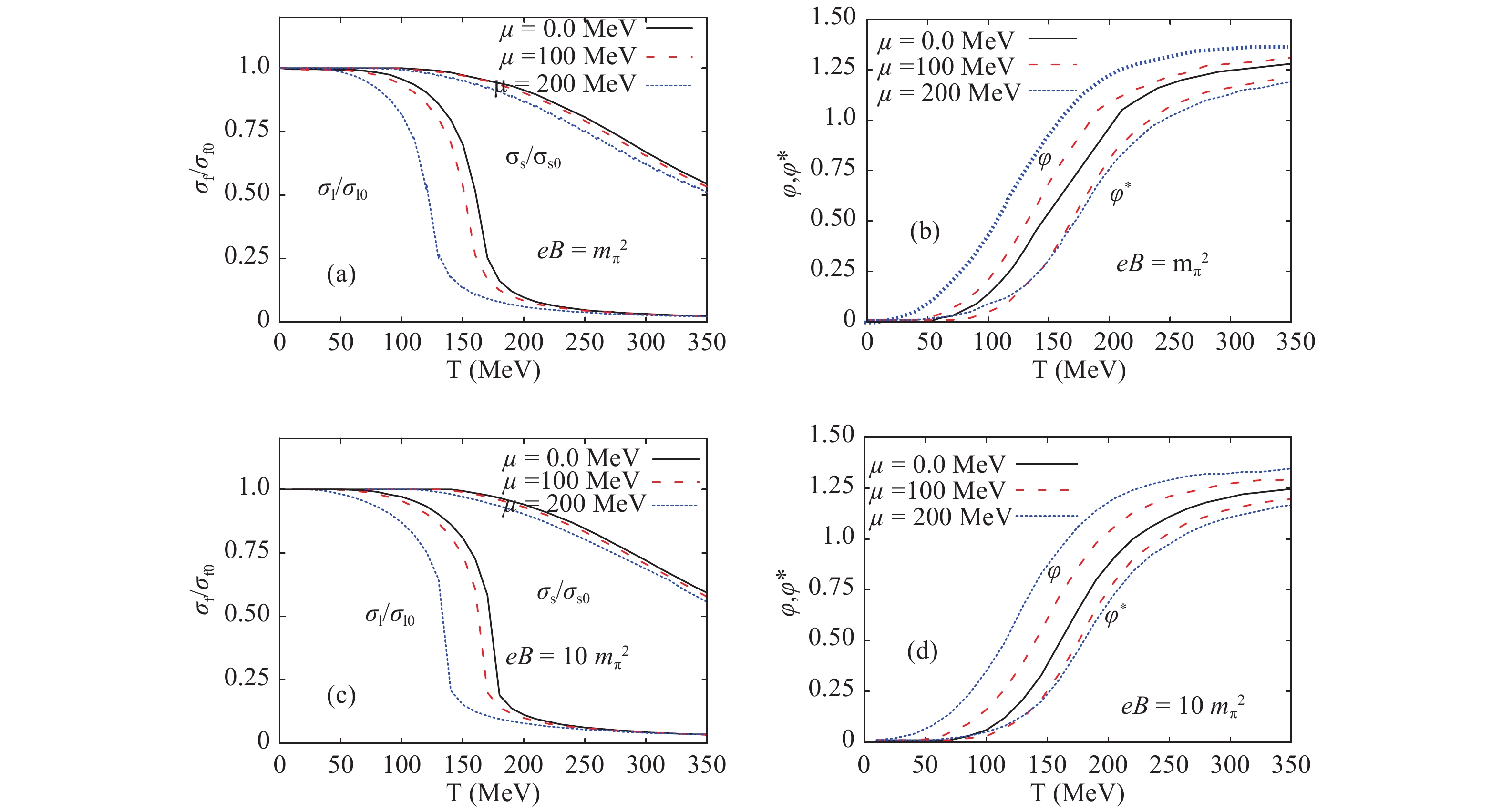Figure1. (color online) Left-hand panels (a) and (c) show the normalized chiral-condensate with respect to the vacuum value as function of temperature. Right-hand panels (b) and (d) show the expectation value of the Polyakov-loop fields ($\phi$ and $\phi^*$) as function of temperature. The top panels present the results for magnetic field $eB =m^2_{\pi}$, while the bottom panels are for $eB=10 \, m^2_{\pi}$. The calculations are performed for different baryon chemical potentials; $\mu=0$ (solid curves), 100 (dashed curves), 200 MeV (dotted curves).

Right-hand panels (b) and (d) show the Polyakov-loop order parameters ($\phi$ and its conjugate $\phi^*$) as function of temperature for the same values of baryon chemical potential and magnetic field as in the left-hand panels. It is obvious that for $\mu=0$ (solid curves), $\phi=\phi ^*$, i.e. the order parameters are indistinguishable. However, they become different for finite $\mu$, $\mu=100$ MeV (dashed curves) and $\mu= 200$ MeV (dotted curves). The effects of the magnetic field are obvious. We observe that the deconfinement critical temperature ($T_{\phi}$) is shifted to lower values as the magnetic field increases, and also as the baryon chemical potential increases. This is similar to the left-hand panels. On the other hand, we conclude that $\phi$ and $\phi^*$ have different dependence on temperature. While $\phi$ increases as the magnetic field increases, and as the baryon chemical potential increases, we find that $\phi^*$ decreases in both cases. Accordingly, the magnetic catalysis related to temperature is respectively a direct or an inverse effect. Again, the determination of $T_{\phi}$ is discussed below.
Figure 2 illustrates the temperature dependence of the normalized chiral quark-condensates (a) and deconfinement order parameters (b) for different magnetic fields, $eB=0$ (solid curves), $0.1$ (dashed curves), $0.2$ (dotted curves) and $0.4$ GeV² (dot-dashed curves), at vanishing chemical potential ($\mu=0$). Relative to the previous figure, this one presents a systematic study of the influence of magnetic fields. In the left-hand panel (a), we find that the critical chiral temperature deceases with increasing magnetic field. This means that the phase transition, which is a crossover, becomes slightly sharper with increasing magnetic field. In the right-hand panel (b), the temperature dependence of the deconfinement order parameters is depicted for a vanishing baryon chemical potential, i.e. $\phi=\phi^*$, but different magnetic field strengths, $eB=0$ (solid curves), $0.1$ (dashed curves), $0.2$ (dotted curves) and $0.4$ GeV² (dot-dashed curves). It is obvious that the critical deconfinement temperature ($T_{\phi}$) decreases very slightly as the magnetic field increases.
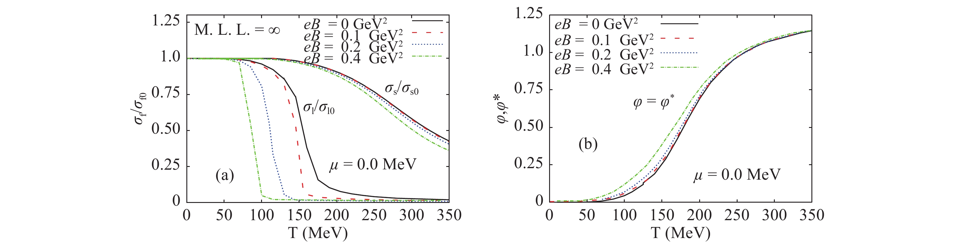Figure2. (color online) Left-hand panel: the normalized chiral condensate as function of temperature for a vanishing baryon chemical potential $\mu=0$ but different magnetic fields, $eB=0$ (solid curves), $0.1$ (dashed curves), $0.2$ (dotted curves) and 0.4 GeV² (dot-dashed curves). Right-hand panel: the same as in the left-hand panel but for the deconfinement order parameters $\phi$ and $\phi^*$.

In both figures, we assure that the maximum Landau levels are fully occupied with quark states. The details about the Landau quantization as a crucial consequence of the magnetic field, and how the corresponding levels are occupied with quark states, can be obtained from Refs. [35, 40].
Furthermore, we have calculated the chiral condensates ($\sigma_l$ and $\sigma_s$) and the deconfinement order-parameters ($\phi$ and $\phi^*$) and their dependence on the baryon chemical potential ($\mu$) for different temperatures and magnetic field strengths. This is illustrated in Fig. 3, for temperatures $T=50$ MeV (top panels) and $T=100$ MeV (bottom panels). In the left-hand panels (a) and (c), the density dependence of the chiral condensates is given as function of different magnetic field strengths, $eB=1$ (solid curves) 10 (dashed curves), 15 (dotted curves), 20 (dot dashed curves), and $25 m^2_{\pi}$ (double dotted curves). We observe that increasing the temperature causes a rapid decrease in the chiral condensates around the chiral phase transition, similar to that observed in a previous study with PLSM without the magnetic field [11] , and in the previous two figures as well. Such a decrease is likely related to a rapid crossover.
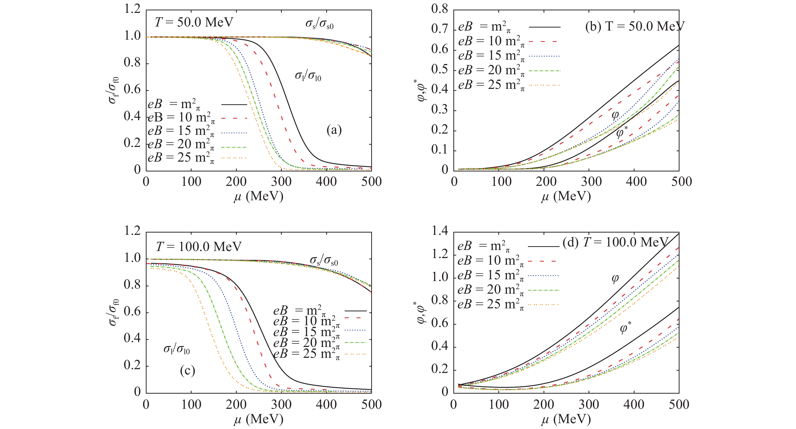Figure3. (color online) Left-hand panels (a) and (c) show the chiral condensates ($\sigma_l$ and $\sigma_s$) normalized to the vacuum value as function of baryon chemical potential for different values of magnetic fields, $eB=1$ (solid curves) 10 (dashed curves), 15 (dotted curves), 20 (dot dashed curves), and $25 m^2_{\pi}$ (double dotted curves). Right-hand panels (b) and (d) show the same as in the left-hand panels but for the expectation value of the Polyakov-loop potentials, i.e. deconfinement order parameters ($\phi$ and $\phi^*$). Top panels show the results for $T=50$ MeV, and bottom panels for $T=100$ MeV.

We observe that increasing the magnetic field accelerates the rapid decrease in the chiral phase-structure. This leads to a decrease in the corresponding critical chemical potential, which is determined in a similar manner as the critical chiral temperature. Increasing the magnetic field tends to accelerate the phase transition, i.e. to accelerate the formation of a metastable phase characterizing the region of crossover. This phenomenon is known as magnetic catalysis, and is actually an inverse one.
There is a gap difference between the light and strange chiral condensates at high densities. This can be understood because of the inclusion of the anomaly term in Eq. (12), which was discussed in Section 2.2, and is known as the c term. The resulting fit parameters are accordingly modified [8, 11]. This was conjectured as an evidence of the numerical estimation of the chiral condensates. The difference between $\sigma_l$ and $\sigma_s$ was also observed in the previous two figures.
The right-hand panels (b) and (d) show the dependence of the deconfinement order parameter on the baryon chemical potential for temperatures $T=50$ (top panel) and $T=100$ MeV (bottom panel), and fixed magnetic field strengths $eB=1$ (solid curves) 10 (dashed curves), 15 (dotted curves), 20 (dot dashed curves), and $25 m^2_{\pi}$ (double dotted curves). The increase in temperature increases the deconfinement order parameters for a larger baryon chemical potential.
It is obvious that the slope of $\phi$ and $\phi^*$ with respect to $\mu$ can be approximately estimated. We observe that the magnetic field decreases both slopes, i.e. increases the corresponding critical chemical potentials, while increasing the temperature increases the slopes and thus decreases the corresponding critical temperatures. Both thermal and magnetic effects of the hadronic medium on the evolution of Polyakov-loop parameters seem to be very smooth.
In light of our study of the phase structure of PLSM for finite T, $\mu$, and $e B$, we can now speculate about the three-dimensional QCD phase-diagram. This was already analyzed in great detail in Ref. [35, 40], where the influence of a finite magnetic field on the QCD phase-diagram, i.e. temperature vs. baryon chemical potential, was analyzed. Interested readers are kindly advised to consult Refs. [35, 40], where T-eB, $\mu$-eB, and T-$\mu$ QCD phase-diagrams are shown. The three-dimensional phase-diagram was depicted as well in [35, 40].
In the present work, we concentrate on a detailed version of the T-eB phase-diagram, Fig. 4. We distinguish between the critical chiral and critical deconfinement temperatures. Also, we confront our calculations to the recent $2+1$ lattice QCD results [41, 42] , and observe excellent agreement.
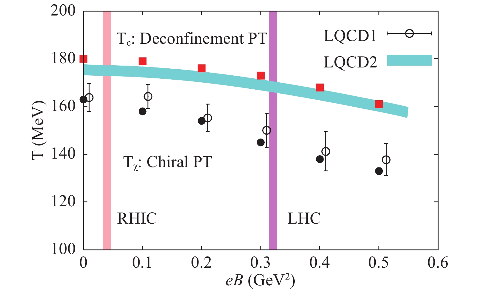Figure4. (color online) Dependence of the critical chiral and critical deconfinement temperatures on a finite magnetic field determined from PLSM (closed symbols). The results are compared to the recent $2+1$ lattice QCD simulations [curve (deconfinement) and open symbols (chiral)] [41, 42]. The vertical bands refer to the estimated averaged magnetic field at RHIC and LHC energies.

Figure 4 illustrates our PLSM estimations of the dependence of the critical chiral and critical deconfinement temperatures, $T_{\chi}$ and $T_c$, on the finite magnetic field. Both chiral (solid circles) and deconfinement (solid rectangles) calculations are confronted to the recent $2+1$ lattice QCD simulations [41, 42]. The open symbols stand for the lattice estimations for $T_{\chi}$, which are determined at the inflection point of the normalized entropy, labeled as LQCD1 [42]. The curved band represents the lattice estimations of the critical deconfinement temperature ($T_c$) at the inflection point of the strange quark-number susceptibility, labeled as LQCD2 [41].
We recall that there are at least two different methods that can be utilized to determine the critical temperature. In the first one, $T_{\chi}$ is calculated using the thermodynamic quantity $s/T^3$, where s is the entropy density. The second one determines $T_c$ as the position where the strange quark-number susceptibility reaches a maximum. It is clear that the PLSM results are in excellent agreement with both lattice QCD predictions [41, 42]. In light of this study, we conclude that both PLSM and lattice QCD simulations clearly indicate that the two types of critical temperatures (chiral and deconfinement) decrease with increasing $e B$, i.e. show the inverse magnetic catalysis.
A few remarks concerning the magnetic catalysis are in order. In Eq. (11), the first term, $U(\sigma_l, \sigma_s)$, refers to the contribution of the valence quarks, the second term, [${\cal{U}}(\phi, \phi^*, T)$] gives the gluonic potential contribution, while the last term [$\Omega_{\bar{q}q} (T, \mu _f, B)$] represents the contribution of the sea quarks. It is well-known that the physical mechanism for magnetic catalysis relies on a competition between valence and sea quarks [43-45]. The mesonic potential has a remarkable effect at very low temperature [30]. In our calculations, we noted that the small value of $U(\sigma_l, \sigma_s)$ leads to an increase in the contribution of the sea quarks. Thus, applying a finite magnetic field results in the suppression of the chiral condensates relevant for restoration of chiral symmetry breaking. This would explain the "inverse magnetic catalysis", which is characterized by a decrease in $T_c$ with increasing magnetic field, as illustrated in Fig. 4, where the critical temperatures of both types of phase transitions decrease with increasing magnetic field. It should be noted that this phenomenon is also observed in the lattice QCD simulations [41, 42].
It is noteworthy to recall that Ref. [46] reported an opposite results, i.e. a direct magnetic catalysis. The first term in the free energy, Eq. (11), $U(\sigma_l, \sigma_s)$, refers to the contribution of the valance quarks. In a previous work [30], we have analyzed the temperature dependence of this specific potential for a vanishing chemical potential. We found that it has a small effect at high temperatures. However, it plays an important role in assuring spontaneous chiral symmetry breaking. PLSM describes the quark-hadron phase structure, where the valence and sea quarks are simultaneously implemented, Eq. (11). We propose that the physical mechanism for magnetic catalysis relies on an interplay between the contributions of sea and valance quarks [43, 45]. We have observed that the magnetic field increasingly suppresses the chiral condensates. Thus, the restoration of chiral symmetry breaking takes place at lower temperatures. Although it is unlikely that the number of the quark flavors alone is sufficient to explain the inverse or usual magnetic catalysis, we emphasize that our calculations assume $2+1$ quarks flavors. For the sake of completeness, we intend in a future work to investigate the magnetic catalysis in SU(4) PLSM, as well.
2 -->

3.2.Chiral phase-structure of meson states in a finite magnetic field

In a previous work, sixteen meson states in thermal and dense medium were studied with SU(3) PLSM [11] for a vanishing magnetic field. For a finite magnetic field, an estimation of the magnetic effects on four meson states was presented in Ref. [31]. In order to conduct a systematic study of the effects of the magnetic field strength on nonet (sixteen) meson states, the chiral phase-structure of each meson-state is analyzed depending on temperature, baryon chemical potential and finite magnetic field.
● We start with an approximate range for the magnetic field strength that may be created in heavy-ion collisions at RHIC and LHC energies [5-7], $eB=1-25 m^2_{\pi}$.
● We then construct the temperature dependence of all meson states corresponding to the lowest Matsubara frequency.
● Last but not least, the chiral phase-structure of the meson states is then given in a wide range of baryon chemical potentials.
In quantum field theory, the hadron mass can be determined from the second derivative of the equation of motion relative to the hadron field of interest. The free energy $\cal{F} (T, \mu, eB, \beta)$ apparently encodes details of the equation of motion, where $\beta$ represents the corresponding meson field. Assuming that the contribution of the quark-antiquark potential to the Lagrangian vanishes in vacuum, the meson potential determines the mass matrix, given as

$ \begin{aligned} m_{i, ab}^2 = \left. \frac{\partial^2 {\cal{F}} (T, \mu, eB, \beta) }{\partial \beta_{i, a} \partial \beta_{i, b} }\right|_{\rm min}, \end{aligned} $

(19)

where i stands for (pseudo)scalar and (axial)vector mesons, and a and b are integers in between 0 and 8. Equation (19) can be split into two different terms.
● The first one is related to vacuum, where the meson masses are derived from the nonstrange ($\sigma_l$) and strange ($\sigma _s$) sigma fields. More details about the estimation of masses in vacuum are given in Appendix A. In this term, the effect of the magnetic field requires numerical estimations for nonstrange and strange sigma-fields.
● The in-medium term, in which the magnetic field is included, reads

$ \begin{split} m_{i, ab}^2 =& \left. \nu_{c}\sum_{f} \frac{|q_f| B T}{(2 \pi)^2} \sum_{\nu = 0}^{\infty} (2-\delta _{0 \nu }) \int_0^{\infty} {\rm d}p_z \right. \\&\times\frac{1}{2E_{B, f}} \biggl[(n_{q, f, B} + n_{\bar{q}, f, B} ) \biggl( m^{2}_{f, a b}-\frac{m^{2}_{f, a} m^{2}_{f, b}}{2 E_{B, f}^{2}} \biggr) \\ & +(b_{q, f, B} + b_{\bar{q}, f, B}) \biggl(\frac{m^{2}_{f, a} m^{2}_{f, b}}{2 E_{B, f} T} \biggr) \biggr], \end{split} $

(20)

where $\nu_c=2 N_c$. This expression gives the meson-mass modifications, which can be estimated from PLSM, Eq. (19), and the diagonalization of the resulting quark-mass matrix. Details about other quantities in Eq. (20) can be obtained in Ref. [9, 11]:
- The quark mass derivative with respect to the meson fields ($\lambda_{i, a}$); $m^2_{f, a} \equiv \partial m^2_f/\partial \lambda_{i, a}.$
- The quark mass with respect to meson fields ($\lambda_{i, a} \partial \lambda_{i, b}$), $m^2_{f, {ab}} \equiv \partial m^2_f/\partial \lambda_{i, a} \partial \lambda_{i, b}$.
- Correspondingly, the antiquark function $b_{\bar{q}, f, B}(T, eB, \mu_f) = b_{q, f, B}(T, eB, -\mu_f)$, where

$ \begin{aligned} b_{q, f, B}(T, eB, \mu_f)= n_{q, f, B}(T, eB, \mu_f) (1-n_{q, f, B}(T, eB, \mu_f)). \end{aligned} $

(21)

- The normalization factors for the quark ($b_{q, f, B}=3(n_{{q}, f} )^2 - c_{q, f, B}$) and antiquark read $b_{\bar{q}, f, B}=3(n_{{\bar{q}}, f, B} )^2 - c_{{{\bar{q}}}, f, B}$,

$ \begin{aligned} n_{q, f, B} =& \frac{\Phi {\rm e}^{- E_{q, f}/T} + 2 \Phi^* {\rm e}^{-2 E_{q, f}/T} + {\rm e}^{-3 E_{q, f}/T}}{1+3(\phi+\phi^* {\rm e}^{-E_{q, f}/T}) {\rm e}^{-E_{q, f}/T}+{\rm e}^{-3E_{\bar{q}, f}/T}}, \end{aligned} $

(22)

$ \begin{aligned} n_{\bar{q}, f, B} =& \frac{\Phi^* {\rm e}^{-E_{\bar{q}, f}/T} + 2 \Phi {\rm e}^{-2E_{\bar{q}, f}/T} + {\rm e}^{-3E_{\bar{q}, f}/T}}{ 1+3(\phi^*+\phi {\rm e}^{-E_{\bar{q}, f}/T}) {\rm e}^{-E_{\bar{q}, f}/T}+{\rm e}^{-3E_{\bar{q}, f}/T}}, \end{aligned} $

(23)

$ \begin{aligned} c_{{q}, f, B} =& \frac{\Phi {\rm e}^{- E_{q, f}/T} +4 \Phi^* {\rm e}^{-2 E_{q, f}/T} +3 {\rm e}^{-3 E_{q, f}/T}}{1+3(\phi+\phi^* {\rm e}^{-E_{q, f}/T}) {\rm e}^{-E_{q, f}/T}+{\rm e}^{-3E_{\bar{q}, f}/T}}, \end{aligned} $

(24)

$ \begin{aligned} c_{\bar{q}, f, B} =& \frac{\Phi^* {\rm e}^{-E_{\bar{q}, f}/T} + 4 \Phi {\rm e}^{-2E_{\bar{q}, f}/T} +3 {\rm e}^{-3E_{\bar{q}, f}/T}}{ 1+3(\phi^*+\phi {\rm e}^{-E_{\bar{q}, f}/T}) {\rm e}^{-E_{\bar{q}, f}/T}+{\rm e}^{-3E_{\bar{q}, f}/T}}. \end{aligned} $

(25)

- The quark and antiquark dispersion relations, $E_{\bar{q}, f}(T, eB, \mu)$ and $E_{q, f}(T, eB, -\mu)$, are equivalent to $E_{B, f}$ in Eq. (14).
It should noted that due to the mixing between the (pseudo)scalar and (axial)vector sectors through the covariant derivative, the tree-level expressions of the pseudoscalars and some scalars are not mass eigenstates. When the corresponding wave functions are renormalized to the constants Z, such a mixing can be resolved. Details can be found in Ref. [25].
3 -->

3.2.1.Dependence of meson states on temperature

Figure 5 shows the (pseudo)scalar and (axial)vector meson states with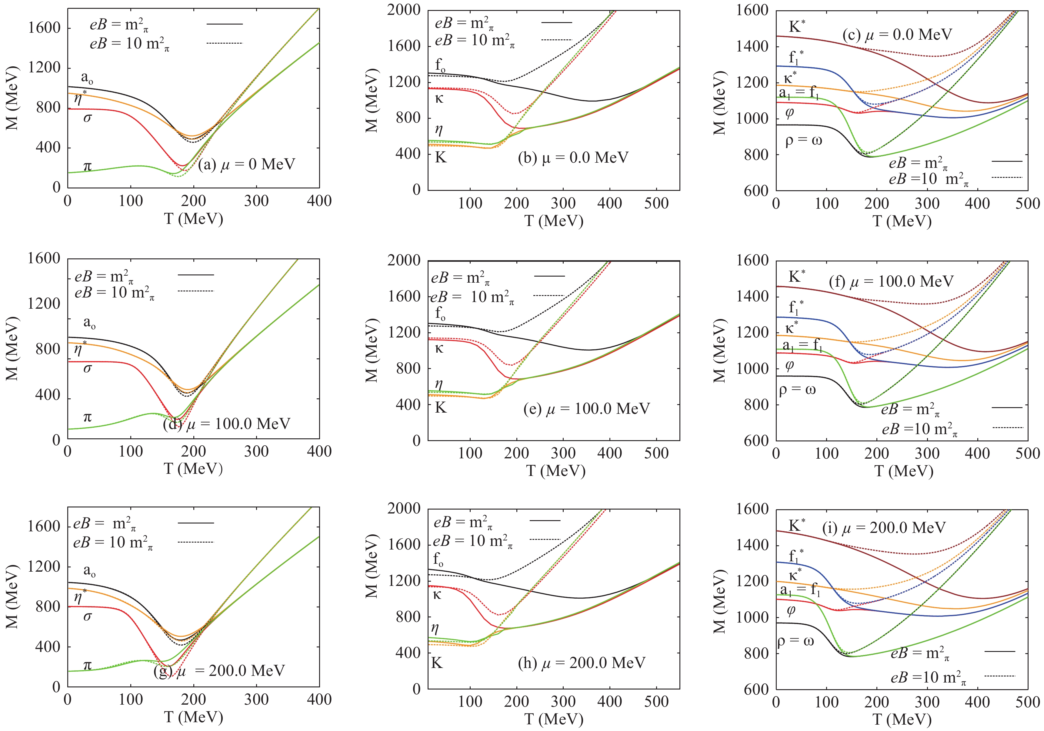 $U(1)_A$-anomaly as function of temperature for a fixed magnetic field strength and fixed baryon chemical potential. The left-hand panels give the $\left[{\rm{a}}_0(980), \sigma(800)\right]$ scalar and $\left[\eta^*(957), {\rm{\pi}}(134) \right]$ pseudoscalar states, while the scalar $\left[f_0(1200), \kappa(1425) \right]$ and pseudoscalar $\left[\eta(547), {\rm{K}}(497)\right]$ meson states are presented in the middle panels. The right-hand panels illustrate the vector $\left[\rho(775), {\rm{K}}^*(891), \omega(782), \phi(1019) \right]$ and axial vector $\left[{\rm{a}}_1(1030), {\rm{f}}_1(1281), {\rm{K}}_1^*(1270), {\rm{f}}_1^*(1420)\right]$ meson states. The solid curves represent the results for $eB=m_{\pi}^2$. The results for $\mu=0.0$ are depicted in the top panels. The middle and bottom panels show the calculations for $\mu=100$ MeV and $\mu=200$ MeV, respectively. The results for $eB=m_{\pi}^2$ are given as dashed curves. To distinguish between such curves, one should note that the curves corresponding to one meson state are usually bundled at low temperatures. At very high temperatures, many, if not all, curves approach asymptotic limits. In the left-hand panels, we observe that increasing magnetic field slightly reduces the meson masses, especially at the critical temperatures. In the middle and right-hand panels, the opposite is obtained, with one exception for Kaons. This might be a subject of an experimental study, especially in the future facilities such as the Facility for Antiproton and Ion Research (FAIR) and the Nuclotron-based Ion Collider fAсility (NICA).
Figure5. (color online) The temperature dependence of (pseduo)scalar and (axial)vector meson states calculated for finite magnetic fields, $eB=m_{\pi}^2$ (solid curves) and $eB=10 m_{\pi}^2$ (dotted curve), at different baryon chemical potentials, $\mu=0$ MeV (top panels), $\mu=100$ MeV (middle panels) and $\mu=200$ MeV (bottom panels).

The mass gap between the various meson states can be estimated from the bosonic thermal contributions. The masses of bosons are given as function of pure sigma fields, the nonstrange ($\sigma_l$) and the strange ($\sigma_s$). At low temperatures, the bosonic thermal contributions are dominant and become stable and finite relative to the corresponding vacuum value of the meson state, until they reach the chiral temperature ($T_{\chi}$) related to the given meson state. At high temperatures, the fermionic (quark) thermal contributions complete the thermal behavior of these states. As they increase with temperature, this leads to degenerate meson masses. It is obvious that the effects of the fermionic (quark) thermal contributions are negligible at low temperatures.
As depicted in Fig. 5, the effects of a finite magnetic field on the thermal contributions of the meson states can be divided into three regions.
● The first region is dominated by the bosonic thermal contributions, and the magnetic field remains ineffective until the second region takes place.
● In the second region, beyond the chiral phase-transition of a given meson state, the influence of the magnetic field becomes obvious. We observe that the increasing magnetic field accelerates the chiral phase-transition of a given meson. By accelerating, we mean that the phase transition takes place at lower temperatures or chemical potentials. As a result, the chiral critical temperature decreases with increasing magnetic field strength.
● The last (third) region represents the fermionic thermal contributions.
We conclude that the magnetic field has an evident effect on quarks and apparently accelerates and sharpens the quark-hadron phase transition.
We observe that at temperatures exceeding the critical values (corresponding to each meson state), the meson masses become degenerate. This can be understood as due to the effect of fermionic fluctuations on chiral symmetry restoration [8], especially on the strange condensate ($\sigma_s$). Such an effect seems to melt the nonstrange condensate ($\sigma_l$) faster than the nonstrange one ($\sigma_l$), Fig. 1. At very high temperatures, the mass gap between mesons seems to disappear due to the melting of the strange condensate ($\sigma_s$). This mass gap appears again at low temperatures, where the nonstrange condensate remains finite. At temperatures higher than critical, only the strange condensate remains finite. These thermal effects are strongly related to the degenerate meson masses.
Also, Fig. 5 shows that the $\sigma$, ${\rm{\pi}}$, ${a}_0$, and $\eta^*$ meson states become degenerate through a first-order phase transition and apparently keep this state at higher temperatures, assuring a completion of the chiral symmetry restoration. The middle panels depict the $\kappa$ meson state and illustrates that it reduces to the $\eta$ and ${K}$ meson states through a first-order phase transition. ${f}_0$ is degenerate at a higher temperature as well through a first-order phase transition. In the right-hand panels, the meson states ${ {f}}_1^*$, $\phi$, ${{a}}_1$, ${{f}}_1$, $\rho$, and $\omega$ become degenerate through chiral phase-transitions, whereas ${{K}}^*$ and $\kappa^*$ become coincident at very high temperatures.
Increasing the baryon chemical potential influences the behavior of the thermal contributions of different meson states as well. We find that the increase of the baryon chemical potential (from top to bottom panels) enhances various degenerate meson masses. For example, the $\sigma$ and ${\rm{\pi}}$ states degenerate at the chiral temperature $T_{\chi}\sim 191.5~$ MeV and $\mu=0~$ MeV. But for $\mu=100~$ MeV, the critical temperature drops to $\sim 186.5~$ MeV , and for $\mu=0~$ MeV, it decreases to $\sim 178.7~$ MeV. Thus, we conclude that the chiral temperature associated to the different meson states decreases with increasing baryon chemical potential. This refers to a remarkable in-medium effect that could be verified in the future facilities with high-density heavy-ion collision experiments.
Our goal is not only the characterization of the meson spectra in thermal and dense medium, but also the description of their vacuum phenomenology in a finite magnetic field. In Table 1, an extensive comparison is given of the results for different scalar and vector meson (nonets) from various effective models, PLSM (present work) and PNJL [12-15, 47] , and from the very recent compilation of PDG [48], lattice QCD calculations [49, 50] and QMD/UrQMD simulations [51]. We conclude that our PLSM calculations are remarkably precise, especially for some light mesons at a vanishing temperature. They are comparable with measurements and lattice calculations, as shall be elaborated in the following section.

sector	meson states	PDG [48]	UrQMD model [51]	present work	PNJL model [12-15, 47]	lattice QCD calculations
						Hot QCD[49]	PACS-CS [50]
scalar $J^{PC}=0^{++}$	${{a}}_{0}$	${{a}}_{0}(980 {\pm 20})$	$984.7$	$1015.73$	837
	$\kappa$	${{K}}_{0}^* (1425 {\pm 50})$	1429	1115	1013
	$\sigma$		$400 - 1200$	800	700
	${{f}}_{0}$	${{f}}_{0}(1281.0 \pm 0.5)$	$1200-1500$	$1102.8$	1169
pseudoscalar $J^{PC}=0^{-+}$	${{\pi}}$	${{\pi}}^0 (134.9770 {\pm 0.0005} )$	$139.57$	$150.4$	126	$134 {\pm 6}$	$135.4 {\pm 6.2}$
	${{K}}$	${{K}}^0$ ($497.611 {\pm 0.013}$)	$493.68$	509	490	$422.6 {\pm 11.3}$	$498 {\pm 22}$
	$\eta$	$\eta(547.862 {\pm 0.17} )$	$517.85$	553	505	$579 {\pm 7.3}$	$688 {\pm 32}$
	$\eta^{'}$	$\eta^{'}(957.78 { \pm 0.06})$	$957.78$	$949.7$	949
vector $J^{PC}=1^{--}$	$\rho$	$\rho(775.26 {\pm 0.25})$	$771.1$	745	$764.08$	$756.2 {\pm 36}$	$597 {\pm 86}$
	$\omega_X$	$\omega (782.65 {\pm 0.12})$	$782.57$	745	$764.08$	$884 {\pm 18}$	$861 {\pm 23}$
	${{K}}^*$	${{K}}^* (891.76 {\pm 0.25})$	$891.66$	894	$899.96$	$1005 {\pm 93}$	$1010.2 {\pm 77}$
	$\omega_y$	$\phi(1019.461 {\pm 0.016})$	$1019.45$	1005	$1025.79$
axial-vector $J^{PC}=1^{++}$	${{a}}_1$	$a_1 (1230 \pm 40)$	1230	980	$1171.78$
	${{f}}_{1x}$	$f_{1}(1281.9 { \pm 0.5})$	$1281.9$	980	$1173.78$
	${{K}}_{1}^{*}$	$K_{1}^{*} (1272 {\pm 7} )$	1273	1135	$1035.21$
	${{f}}_{1y}$	$f_{1}^{'}(1426.4 {\pm 71.30.9})$	1512	1315	$1531.55$

Table1.Comparison of the (pseudo)scalar and (axial)vector meson states obtained in the present work (PLSM), and the corresponding results from PNJL [13-15], the latest compilation of PDG [48], QMD/UrQMD [51] and lattice QCD calculations [49, 50].

Only pseudoscalar and vector meson sectors are available from HotQCD [49] and PACSCS collaborations [50]. It is obvious that our estimations for meson masses agree well with previous calculations [8, 9, 11, 25] for mixing strange with nonstrange scalar states, where it was reported that one gets various states below 1 GeV and one above 1 GeV [25]. The agreement between PLSM and the available lattice-calculations is excellent.
3 -->

3.2.2.Dependence of meson states on baryon chemical potential

Figure 6 shows the dependence of scalar and vector meson states (labeled curves) on the baryon chemical potentials in the presence of the U(1)_A anomaly, for magnetic fields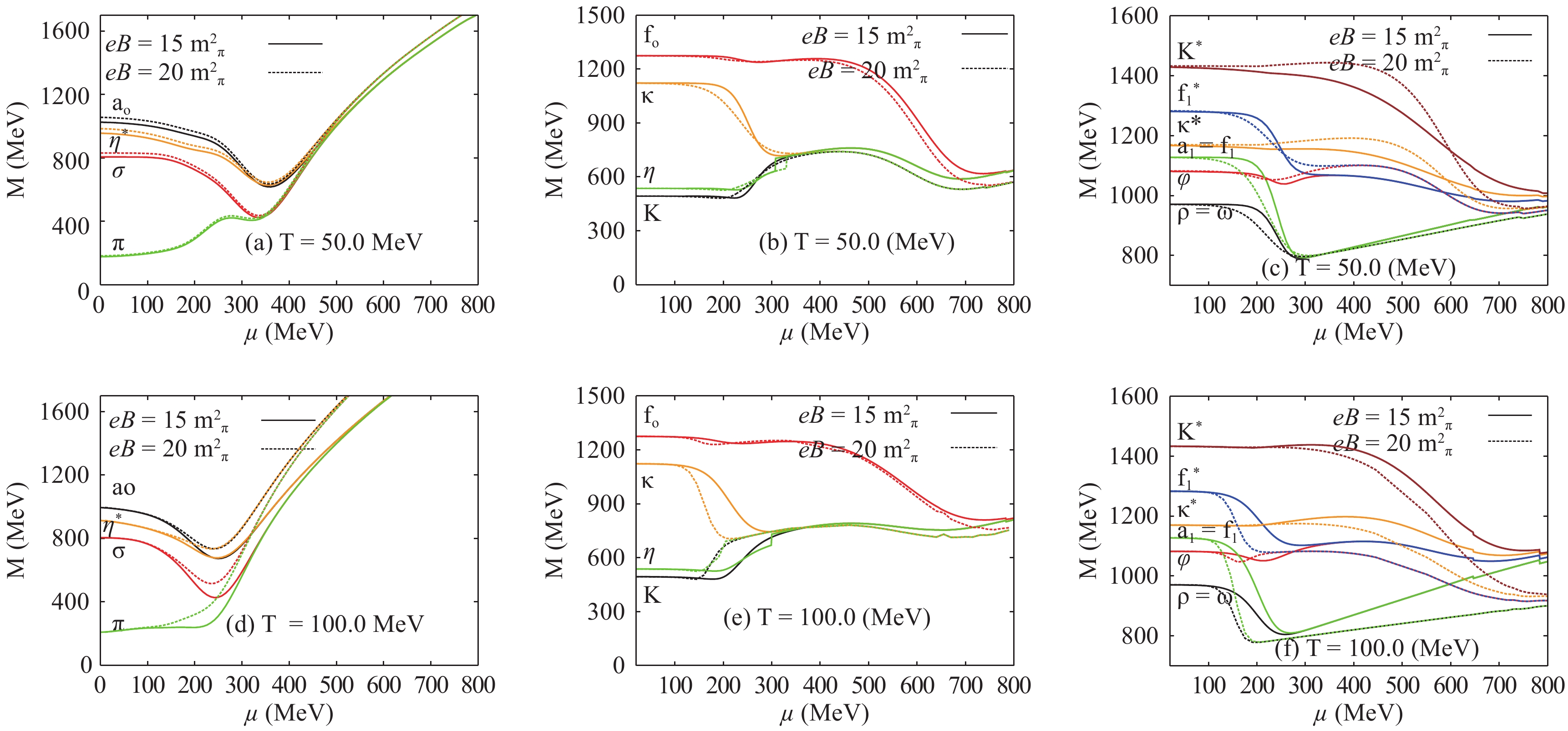 $eB=15 m_{\pi}$ (solid curves) and $eB=20 m_{\pi}$ (dashed curves), and temperatures $T=50$ (top panel), and 100 MeV (bottom panel). As discussed in previous sections, the nonstrange ($\sigma_l$) and strange quark ($\sigma_s$) chiral condensates strongly depend on the temperature and baryon chemical potential. The mass gap which distinguishes between the meson states results from dense bosonic contributions. Such contributions remain independent on the baryon chemical potential until they reach the Fermi surface [11, 52]. The masses are then liberated through a first-order phase transition. To assure that the Polyakov-loop potentials include the deconfinement phase transition in LSM, the dynamics of color charges was included as a new type of interaction. Apparently, the meson masses remain degenerate through the deconfinement phase transition. When comparing these results with our previous ones [11], we conclude that the deconfinement phase transition in the present work, where a finite magnetic field is included, seems to become sharper and faster, i.e. the region of $\mu$ within which the masses of the meson states decrease, indicating a rapid change in the underlying dynamics and degrees of freedom, becomes narrower as the magnetic field is increased. This finding could be a subject of a future experimental verification.
Figure6. (color online) Dependence of the masses of (pseudo)scalar and (axial)vector meson states on the baryon chemical potential for magnetic field strengths $eB=15\, m_{\pi}^2$ (solid curves) and $eB=20\, m_{\pi}^2$ (dotted curve), and temperatures $T=50~$ MeV (top panels) and $T=100~$ MeV (bottom panels).

Another finding of the present work is that for a fixed magnetic field, the finite baryon chemical potential is conjectured to contribute through baryon density to the masses of various meson states, and is dominant in three regions:
● The first region is characterized by low $\mu$, where the gap difference between the meson masses seems to originate in dense bosonic contributions. These are obtained from the mesonic Lagrangian of LSM.
● The second region appears when the meson states undergo a chiral phase-transition from confined hadron phase to parton phase, where quarks and gluons dominate the underlying degrees of freedom.
● The third region is characterized by large $\mu$, where the hadrons are conjectured to dissolve into their constituent free quarks and gluons.
As was obtained in the study of the temperature dependence, the dependence of various meson masses on $\mu$ is accompanied by a decrease of the bosonic contributions to the medium density, which become negligible at very large baryon chemical potentials. In this limit, the dense fermionic contributions become dominant. Furthermore, the latter lead to mass degeneration, which takes place through dense fermionic contributions. Accordingly, the meson states, if they pass through the phase transition as bound hadron states or survive the critical density ($\mu_{\rm{crit}}$) at which the phase transition takes place, rely on dense fermonic contributions to overcome the energy gap of the Fermi surfaces. The latter differs from one meson state to another. With increasing $\mu$, the bound meson states are assumed to be free and entirely converted into deconfinment (partonic) phase [11, 52].
In the middle panels of Fig. 6, we note that the meson masses reduce in the first-order phase transition. Concretely, the mass of the $\kappa$ state reduces to the masses of ${ {K}}$ and $\eta$ states at $\mu_{\rm{crit}} \sim 350~$ MeV. The temperature is fixed at $50~$ MeV. It seems that the ${\rm{f}}_0$ meson state has a stronger Fermi surface because of the strange quarks. The mass of this state seems to survive until $\mu \sim 500~$ MeV. At $T=100$ MeV (bottom panel), the first-order phase transition seems to persist for small $\mu$. The mass of $\kappa$ reduces to the masses of ${{K}}$ and $\eta$ states at $\mu_{\rm{crit}} \sim 298$ MeV for the magnetic field $eB=15 m_{\pi}^2$ , and $\mu_{\rm{crit}} \sim 200~$ MeV for $eB=20 m_{\pi}^2$. Also, the mass of $f_0$ meson degenerates at lower $\mu_{\rm{crit}}$ than at $T=50$ MeV (top panel).
In Fig. 6, two independent quantities (T and $e B$) have non-negligible effects on the dependence of meson masses on $\mu$. From the QCD phase-diagram [31, 32] and the chemical freezeout boundary [53], we conclude that increasing T reduces $\mu_{\rm{crit}}$. Our results also show that increasing T reduces $\mu_{\rm{crit}}$, at which the bosonic contribution for a finite chemical potential becomes small. Increasing $\mu$ has an obvious influence on scalar mesons, as reaching stable levels of meson masses is accelerated. These are the levels at which the meson masses no longer depend on $\mu$. Concretely, we observe that the masses of vector mesons stay nearly constant until the phase transition takes place, while the masses of axial vector mesons show stronger melting above the Fermi surface. Furthermore, increasing $e B$ is assumed to reduce $\mu_{\rm{crit}}$ and thus to enhance the chiral phase-transition, which explains the influences of finite $e B$ on the $\mu$ dependence of various meson states.
3 -->

3.2.3.Meson states normalized to the lowest Matsubara frequency

In thermal field theory, the Matsubara frequencies are considered as a summation over all discrete imaginary frequencies

$ \begin{aligned} S_{\pm} =& T \sum_{i \omega_n} g(i \omega_n), \end{aligned} $

(26)

where $\pm$ stands for bosons and fermions, respectively, and $g(i \omega_n)$ is a rational function, where $\omega_n=2 n \pi T$ and $\omega_n=(2 n+1) \pi T$ represent bosons and fermions, respectively. The integers $n=0, \pm 1, \pm 2, \cdots$ play an important role in the quantization process. Using the Matsubara frequency, the weighting function $\Gamma_{\eta}(z)$ has two poles at $z=i \omega_n$. Then

$ \begin{aligned} S_{\pm} =& \frac{T}{2 \pi i} \oint g(z) \Gamma_{\eta}(z) {\rm d} z. \end{aligned} $

(27)

$\Gamma_{\pm}(z)$ can be chosen depending on which half plane the convergence is to be controlled in,

$ \begin{aligned} \Gamma_{\pm}(z) =& \left\{\begin{array}{l} \eta \displaystyle\frac{1+n_{\pm}(z)}{T} \\ \\ \eta \displaystyle\frac{n_{\pm}(z)}{T} \end{array} \right., \end{aligned} $

(28)

where the single particle distribution function is given as $n_{\pm}(z)=(1\pm e^{z/T})^{-1}$.
The boson masses are conjectured to get contributions from the Matsubara frequencies [54]. Furthermore, at temperatures above the chiral phase-transition ($T\geqslant T_c$), the thermal behavior of the thermodynamic quantities, such as susceptibilities, and of the masses are affected by the interplay between the lowest Matsubara frequency and the Polyakov-loop potentials [55]. In light of the latter, we apply a normalization of the present meson sectors with respect to the lowest Matsubara frequency, which is associated to bosons $2 \pi T$ [56]. This allows to define the dissolving critical temperature at which the various meson states are conjectured to liberate into the degrees of freedom of free quarks and free gluons. We found that different meson states have different dissolving temperatures, which means that different hadrons, in this case mesons, have different chiral critical temperatures ($T_{\chi}$). In other words, not all hadrons melt into a quark-gluon plasma simultaneously.
Figure 7 depicts the normalization of the different meson states with respect to the lowest, in this case bosonic, Matsubara frequency ($2 \pi T$) for a vanishing (top panel) and finite baryon chemical potential (bottom panel), and different magnetic fields $eB=m_{\pi}^2$ (solid curves) and $eB=10 m_{\pi}^2$ (dotted curves). The legends are identical to those in previous figures. It is obvious that the masses of almost all meson states become independent of temperature, i.e. construct a kind of a universal curve, especially at high temperatures. This observation is a clear signature of dissociation of mesons, which are apparently dissolving into free quarks and gluons. Also, it is found that the characteristic critical temperature does not seem to be universally valid for all meson states. As discussed in earlier sections, the two thermodynamics variables, temperature and magnetic field, seem to enhance the chiral phase-transition and therefore have a considerable influence on the corresponding critical temperature. This observation is also confirmed here.
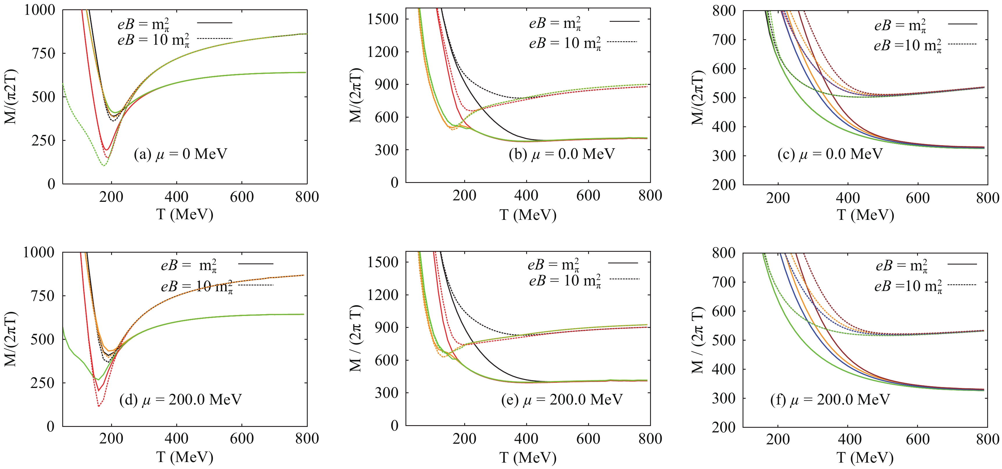Figure7. (color online) Left-hand and middle panels depict the scalar and pseudoscalar meson sectors, respectively, as function of temperature for vanishing (top panels) and finite baryon chemical potential (bottom panels). The right-hand panel shows the same as in the left-hand panel but for vector and axial vector meson sectors.

Table 2 summarizes the different meson states and their approximate dissolving critical temperatures ($T_c^d$) for the finite magnetic field $eB=m_{\pi}^2$ and vanishing baryon chemical potential. The magnetic field strength $eB=m_{\pi}^2$ is likely to be generated at the top RHIC energy. The critical temperatures $T_c^d$ can roughly be read off from the resulting graph. Statistical uncertainties (errors) have not yet been estimated. As mentioned, different meson states seem to have different dissolving temperatures. This is a novel observation of the present work. To connect the latter with the critical temperatures, the first principle lattice calculations should be first reproduced by our QCD-like calculations. The experimental results should be verified as well. It should be noted that our calculations are based on PLSM, a QCD-like model in which not all aspects of QCD are taken into account. Nevertheless, PLSM as such seems to give a good picture of what lattice QCD simulations produce. As an outlook, we plan to devote a future work to a systematic analysis of the resulting dissolving temperatures at varying magnetic fields. The latter can be obtained at different beam energies and in different heavy-ion collision centralities, especially in the future facilities which will enable to cover the gap at high densities.

comparison	scalar mesons	pseudoscalar mesons	vector mesons	axial vector mesons
meson states	$a_{0} \; \kappa\; \sigma \; f_{0}$	$\pi \; K \; \eta \; \eta ^{'}$	$\rho \; K _{0}^{*} \; \omega \; \phi$	$a_{1} \; K_1 \; f_1 \; f_1^*$
$T_{c}^{d}$ in MeV	$430 \; 450 \; 470 \; 450$	$320 \; 230 \; 335 \; 240$	$495 \; 495 \; 495 \; 495$	$495 \; 495 \; 495 \; 495$

Table2.Approximate dissolving critical temperatures, $T_c^d$, corresponding to different meson states at $eB=m_\pi^2$. Statistical uncertainties (errors) have not yet been estimated.

The present study aims at a systematic investigation of the temperature and chemical potential dependence of sixteen meson states [pseudoscalars ($J^{pc}=0^{-+}$), scalars ($J^{pc}=0^{++}$), vectors ($J^{pc}=1^{--}$) and axial-vectors ($J^{pc}=1^{++}$)] constructed from the SU(3) Polyakov linear-sigma model in the presence of finite magnetic fields. The introduction of magnetic fields in this QCD-like model is accompanied by certain modifications in the phase space and in the dispersion relations, among others. Also, this requires Landau quantization to be implemented, for which we use the Landau theory for quantized cyclotron orbits of charged particles in an external magnetic-field. Consequently, some restrictions are added to the color and electric charges of the quarks.
In relativistic heavy-ion collisions, a huge magnetic field is expected. For instance, due to oppositely directed relativistic motion of charges (spectators) in peripheral collisions and/or due to the local momentum-imbalance of the participants in central collisions, a huge magnetic field can be created. To get a picture of its magnitude, we recall that at SPS, RHIC and LHC energies, the strength of such fields ranges between $0.1$ to 1 to $10-15 m_{\pi}^2$, respectively, where $m_{\pi}^2 \sim 10^8~$Gauss. In light of these estimates, studying the possible influence of the magnetic field on QCD matter is of great interest for our understanding of heavy-ion collisions, and, therefore, it increasingly gains popularity among particle physicists.
In the mean-field approximation of PLSM, a grand canonical partition function can be constructed. In order to prepare for the proposed calculations, we have to estimate the temperature dependence of the deconfinement ($\phi$ and $\phi^*$) and chiral order parameters ($\sigma_l$ and $\sigma_s$) in presence of a finite magnetic field. We have found that, taking into consideration the influence of finite magnetic fields, these parameters strongly affect the entire QCD phase transition.
In a previous work, we have studied the distribution of Landau levels and showed how they are occupied for finite magnetic field, temperature, and baryon chemical potential [35, 40]. We concluded that the occupation of each Landau level varies with quark electric charge, as well as with temperature and baryon chemical potential. This is assumed to be characterized by the QCD energy scale.
In PLSM with mean-field approximation, the masses can be determined from the second derivative of free energy with respect to the corresponding hadron field, evaluated at its global minimum. We have presented the temperature and chemical potential dependence of sixteen SU(3) meson masses in finite magnetic fields. For a finite magnetic field, the broken chiral-symmetry is assumed to contribute to the mass spectra. We utilize this assumption to define the chiral phase structure of nonet meson sectors as function of temperature and chemical potential. We found that the spectra of meson masses can be divided into three regions.
● At small temperatures and baryon chemical potentials, the first region is related to the bosonic contributions which are apparently stable.
● The second region is the chiral phase transition, which seems to have a remarkable influence related to the finite magnetic field. It is obvious that the finite magnetic field improves, i.e. sharpens and accelerates, the chiral phase transition of a given meson state.
● The third region is characterized by fermionic contributions, which increase with increasing temperature.
We conclude that the thermal bosonic (meson) mass contributions decrease with increasing temperature. The fermionic (quark) contributions considerably increases at high temperatures. At low temperatures, bosonic contributions become dominant and reach a kind of a stable plateaus relative to the vacuum mass of each meson sector. In this temperature limit, the effects of fermionic contributions are negligibly small. It is noteworthy to highlight that the bosonic contributions result in the mass gap between different meson states in thermal and dense medium. With increasing temperature, the fermionic contributions complete the thermal behavior of these states and lead to mass degeneracy at very high temperatures.
From the scalar and vector mesons normalized to the lowest Matsubara frequency, we also conclude that a rapid decrease of their masses is observed as the temperature increases. Starting from the critical temperature corresponding to each meson sector, we find that the temperature dependence almost vanishes. At high temperatures, we note that the masses of almost all meson states become temperature independent, i.e. they construct a kind of a universal line. This is to be seen as a signature of dissolving of confined mesons into colored quarks and gluons. In other words, the meson states undergo different deconfinement phase transitions, i.e. the various hadrons very likely have different critical temperatures. This is one of the essential findings of the present study, to be confirmed by first-principle lattice simulations and ultimately in future experiments.
We have compared our calculations for scalar and vector mesons with the latest compilation of PDG, lattice QCD calculations and QMD/UrQMD simulations, and found that our results are remarkably precise, especially for some light mesons at vanishing temperature. This implies that the parameters of the QCD-like model we have utilized are reliable.

In vacuum, the mesonic sectors are formulated independently for nonstrange and strange fields:
● For scalar meson states, the squared masses for the scalar sector ($i=S$) are given as

$ \tag{A1} \begin{aligned} m^2_{a_0} =& m^2 + \lambda_1 \left( {\bar{\sigma}} _l^2 + {\bar{\sigma}} _s^2\right) + \frac{3 \lambda_2}{2} {\bar{\sigma}} _l^2 +\frac{\sqrt{2} c}{2} {\bar{\sigma}} _s, \end{aligned} $

$ \tag{A2} \begin{aligned} m^2_{\kappa} =& m^2 + \lambda_1 \left( {\bar{\sigma}} _l^2 + {\bar{\sigma}} _s^2\right) + \frac{\lambda_2}{2} \left( {\bar{\sigma}} _l^2 + \sqrt{2} {\bar{\sigma}} _l {\bar{\sigma}} _s + 2 {\bar{\sigma}} _s^2\right) + \frac{c}{2} {\bar{\sigma}} _l, \end{aligned} $

$ \tag{A3} \begin{aligned} m^2_\sigma =& m^2_{S, {00}} \cos^{2}\theta _S + m^2_{S, {88}}\sin^{2}\theta_S + 2 m^2_{S, {08}} \sin \theta_S \cos \theta_S, \end{aligned} $

$ \tag{A4} \begin{aligned} m^2_{f_0} =& m^2_{S, {00}} \sin^{2}\theta _S + m^2_{S, {88}}\cos^{2}\theta_S - 2 m^2_{S, {08}} \sin \theta_S \cos \theta_S, \end{aligned} $

with

$ \begin{aligned} m^2_{S, {00}} =& m^2 + \frac{\lambda_1}{3} \left(7 {\bar{\sigma}} _l^2 + 4 \sqrt{2} {\bar{\sigma}} _{l} {\bar{\sigma}} _{s} + 5 {\bar{\sigma}} _s^2\right) \\&+ \lambda_2\left( {\bar{\sigma}} _l^2 + {\bar{\sigma}} _s^2\right) -\frac{\sqrt{2}c}{3}\left(\sqrt{2} {\bar{\sigma}} _l + {\bar{\sigma}} _s\right), \\ m^2_{S, {88}} =& m^2 + \frac{\lambda_1}{3} \left(5 {\bar{\sigma}} _l^2 - 4 \sqrt{2} {\bar{\sigma}} _{l} {\bar{\sigma}} _{s} + 7 {\bar{\sigma}} _s^2\right) \\&+ \lambda_2\left(\frac{ {\bar{\sigma}} _l^2}{2} + 2 {\bar{\sigma}} _s^2\right) +\frac{\sqrt{2}c}{3}\left(\sqrt{2} {\bar{\sigma}} _l - \frac{ {\bar{\sigma}} _s}{2}\right), \\ m^2_{S, {08}} =& \frac{2 \lambda_1}{3}\left(\sqrt{2} {\bar{\sigma}} _l^2 - {\bar{\sigma}} _l {\bar{\sigma}} _s - \sqrt{2} {\bar{\sigma}} _s^2 \right) \\&+ \sqrt{2}\lambda_2 \left(\frac{ {\bar{\sigma}} _l^2}{2} - {\bar{\sigma}} _s^2 \right) + \frac{c}{3\sqrt{2}} \left( {\bar{\sigma}} _l - \sqrt{2} {\bar{\sigma}} _s\right). \end{aligned} $

● For pseudoscalar meson states, the squared masses for the pseudoscalar sector ($i=p$) read

$ \tag{A5} \begin{aligned} m^2_\pi =& m^2 + \lambda_1 \left( {\bar{\sigma}} _l^2 + {\bar{\sigma}} _s^2\right) + \frac{\lambda_2}{2} {\bar{\sigma}} _l^2 -\frac{\sqrt{2} c}{2} {\bar{\sigma}} _s, \end{aligned} $

$ \tag{A6} \begin{aligned} m^2_K =& m^2 + \lambda_1 \left( {\bar{\sigma}} _l^2 + {\bar{\sigma}} _s^2\right) + \frac{\lambda_2}{2} \left( {\bar{\sigma}} _l^2 - \sqrt{2} {\bar{\sigma}} _l {\bar{\sigma}} _s + 2 {\bar{\sigma}} _s^2\right) - \frac{c}{2} {\bar{\sigma}} _l, \end{aligned} $

$ \tag{A7} \begin{aligned} m^2_{\eta'} =& m^2_{p, {00}} \cos^{2}\theta _p + m^2_{p, {88}}\sin^{2}\theta _p + 2 m^2_{p, {08}} \sin \theta _p \cos \theta_p, \end{aligned} $

$ \tag{A8} \begin{aligned} m^2_{\eta} =& m^2_{p, {00}} \sin^{2}\theta_p + m^2_{p, {88}}\cos^{2}\theta_p - 2 m^2_{p, {08}} \sin \theta_p \cos \theta_p, \end{aligned} $

with

$ \begin{aligned} m^2_{p, {00}} =& m^2 + \lambda_1 \left( {\bar{\sigma}} _l^2 + {\bar{\sigma}} _s^2\right) + \frac{\lambda_2}{3}\left( {\bar{\sigma}} _l^2 + {\bar{\sigma}} _s^2\right) +\frac{c}{3}\left(2 {\bar{\sigma}} _l + \sqrt{2} {\bar{\sigma}} _s\right), \\ m^2_{p, {88}} =& m^2 + \lambda_1 \left( {\bar{\sigma}} _l^2 + {\bar{\sigma}} _s^2\right) + \frac{\lambda_2}{6}\left( {\bar{\sigma}} _l^2 + 4 {\bar{\sigma}} _s^2\right) -\frac{c}{6}\left(4 {\bar{\sigma}} _l - \sqrt{2} {\bar{\sigma}} _s\right), \\ m^2_{p, {08}} =& \frac{\sqrt{2} \lambda_2}{6} \left( {\bar{\sigma}} _l^2 - 2 {\bar{\sigma}} _s^2\right) - \frac{c}{6}\left(\sqrt{2} {\bar{\sigma}} _l - 2 {\bar{\sigma}} _s\right), \end{aligned} $

and the mixing angles are given by

$ \tag{A9} \begin{aligned} \tan 2\theta_i =& \frac{2 m^2_{i, {08}}}{m^2_{i, {00}}-m^2_{i, {88}}}\ , \ i=S, p\ . \end{aligned} $

● For vector meson states, the squared masses for the vector sector ($i=V^{\mu}$) can be expressed as

$ \tag{A10} \begin{aligned} m_{\rho}^{2} =&m_{1}^{2}+\frac{1}{2} \left(h_{1}+h_{2}+h_{3}\right) {\bar{\sigma}} _l^{2} +\frac{h_{1}}{2} {\bar{\sigma}} _s^{2}+2\delta_{l}, \end{aligned} $

$ \tag{A11} \begin{split} m_{K^{\star}}^{2} =&m_{1}^{2}+\frac{ {\bar{\sigma}} _l^{2}}{4} \left(g_{1}^{2}+2h_{1} +h_{2}\right) \\&+\frac{ {\bar{\sigma}} _l {\bar{\sigma}} _s}{\sqrt{2}}(h_{3}-g_{1}^{2})+\frac{ {\bar{\sigma}} _s^{2}}{2}\left(g_{1}^{2}+h_{1}+h_{2}\right)+\delta_{l}+\delta_{s}, \end{split} $

$ \tag{A12} \begin{aligned} m_{\omega_{x}}^{2} =&m_{\rho}^{2}, \end{aligned} $

$ \tag{A13} \begin{aligned} m_{\omega_{y}}^{2} &=&m_{1}^{2}+\frac{h_{1}}{2} {\bar{\sigma}} _l^{2} + \left( \frac{h_{1}}{2}+h_{2}+h_{3}\right) {\bar{\sigma}} _s^{2}+2\delta_{s}, \end{aligned} $

● And finally, for axial-vector meson states, the squared masses for the axial-vector sector ($i=A^{\mu}$) are

$ \tag{A14} m_{a_{1}}^{2} =m_{1}^{2}+\frac{1}{2} \left(2g_{1}^{2}+h_{1}+h_{2}-h_{3}\right) {\bar{\sigma}} _l^{2}+\frac{h_{1}}{2} {\bar{\sigma}} _s^{2}+2\delta_{l}, $

$ \tag{A15} \begin{split} m_{K_{1}}^{2} =&m_{1}^{2}+\frac{1}{4}\left( g_{1}^{2}+2h_{1}+h_{2}\right) {\bar{\sigma}} _l^{2}-\frac{1}{\sqrt{2}} {\bar{\sigma}} _l {\bar{\sigma}} _s \left(h_{3}-g_{1}^{2}\right) \\&+ \frac{1}{2}\left(g_{1}^{2}+h_{1}+h_{2}\right) {\bar{\sigma}} _s^{2} +\delta_{l}+\delta_{s}, \end{split} $

$ \tag{A16} m_{f_{1x}}^{2} = m_{a_{1}}^{2}, $

$ \tag{A17} m_{f_{1y}}^{2}=m_{1}^{2}+\frac{ {\bar{\sigma}} _l^{2}}{2} h_{1}+\left(2g_{1}^{2}+\frac{h_{1}}{2}+h_{2}-h_{3}\right) {\bar{\sigma}} _s^{2}+2\delta_{s}. $