HTML
--> --> -->There are two basic cycle strategies for RRC systems that specify how ICs are produced in the RM: full cycle (FC, i.e., continuous cycle) and partial cycle (PC). The FC strategy was used by early RRC systems such as the RUC (Rapid Update Cycle) (Benjamin et al., 2004a, b). It uses the ICs directly from the predictions of the previous cycle but slightly adjusted by recent observations using various data assimilation (DA) algorithms, such as the three-dimensional variation (3D-Var) (Benjamin et al., 2004a, b), the Ensemble Kalman Filter (EnKF) (Schwartz and Liu, 2014) and the hybrid variational-ensemble (Schwartz and Liu, 2014; Schwartz et al., 2015). Hence, the regional model in FC mode reaches balance very quickly at the beginning of every cycle, which means a “warm restart”. The global model (GM) just provides the initial field of the first cycle and the cyclically updated lateral and lower boundary conditions (LBCs). The development of synoptic and convective systems in an FC strategy can be regulated by DA and the updated LBCs. However, the FC strategy is limited by the accumulated error from the LBCs using the Newton relaxation method (Davies, 1976) and from the physical parameterizations (Kanamaru and Kanamitsu, 2007; Awan et al., 2011). These biases can hinder correct longwave representation in RMs (Miguez-Macho et al., 2004; Cha and Lee, 2009; Vincent and Hahmann, 2015; Benjamin et al., 2016), cause small-scale convective systems to lose predictability within the short term via an energy cascade process (Durran and Gingrich, 2014; Durran and Weyn, 2016), and accumulate errors cycle by cycle during a continuous run, resulting in reduced forecast performance (Guidard and Fischer, 2008). DA is not very effective in rectifying the bias because it cannot include the set of observations outside the limited regional domain (Guidard and Fischer, 2008; Benjamin et al., 2016). In turn, this bias can weaken the effectiveness of DA by providing inaccurate background fields (Sun et al., 2012). Besides, the DA in RMs cannot make as good use of the satellite data as global DA systems and would retain large systematic errors over marine areas (Hsiao et al., 2012).
To address this limitation, many recently developed RRC systems (Hsiao et al., 2012; Sun et al., 2012; Benjamin et al., 2016; Tong et al., 2016) instead use the PC strategy, which intermittently re-initializes the RM from a GM forecast every several cycles. Typically, a 3–6-hour spin-up is necessary to reach a stable model balance, which means a “cold restart” occurs at the beginning of these re-initialization cycles. Given that a GM has no LBCs, the large-scale error from LBCs can be periodically mitigated. In a PC RRC, the development of the synoptic and convection systems is regulated not only by DA and LBCs but also by reinitialized ICs. The high-resolution convective systems are regenerated from scratch during the restart time. Although the PC strategy has been reported to perform better than the FC strategy (Benjamin et al., 2016), such a “cold restart” process causes two problems. First, the frequent re-initialization in the PC strategy consumes more computing resources than the FC. It is difficult to re-initialize the RM every cycle, especially for RRCs with a short updating interval, such as 12-hour (Sun et al., 2012; Benjamin et al., 2016) or 24 h (Tong et al., 2016; Xie et al., 2019). As a result, large-scale biases from GMs can still accumulate during the cycles that are not re-initialized. Second, forecast precipitation patterns may become discontinuous at re-initialization time, as the generated small-scale systems are not related to their counterparts in the previous cycle. Although previous studies have tried to re-initialize the RRC at a time with climatologically stable weather such as midnight (Hsiao et al., 2012; Tong et al., 2016), there rarely exists a common “stable weather time” over a large domain with various climatic zones. For example, in the mountainous areas of China, convection is triggered by strong latent heating and the enforced uplift even at midnight (Xu and Zipser, 2011; Zhu et al., 2018).
Therefore, operational RRC needs a strategy that can re-introduce the large-scale information from GM every cycle without the spin-up process, i.e., a warm rather than a cold restart. The method should mitigate the bias of RRC more by adjusting the initial large-scale pattern and contaminate the RM balance less. Previous studies have used various schemes to introduce the large-scale information from GM fields into RM (Yang, 2005a, b; Guidard and Fischer, 2008; Stappers and Barkmeijer, 2011; Wang et al., 2014; Yue et al., 2018). One effective method is blending, which combines the low-pass-filtered GM fields with high-pass-filtered RM fields using a Raymond filter (Raymond, 1988). Previous studies have reported improvements in forecasted state variables and precipitation using this method (Yang, 2005a, b; Stappers and Barkmeijer, 2011; Wang et al., 2014; Hsiao et al., 2015). Recently, Feng et al. (2020) updated the blending method to a dynamic blending (DB) scheme to select the large-scale spectrum from the GM forecasts with a time-varied cut-off scale, which indicates the wavebands to be blended. Batch experiments in an RRC over the western continental United States gave encouraging results. DB not only reduces the RM bias on the largescale waveband but adds less small-scale noise to the blended fields. Although the study still retained the spin-up process and did not use DA, it suggested the possible return to FC strategy using the scheme.
Using DB and DA to adjust the initial fields in every cycle, we implement a new FC strategy in an RRC named Rapid-refresh Multi-scale Analysis and Prediction System for Short-Term weather (RMAPS-ST) for the weather forecast in China. This new FC strategy is applied to 7-day cycled forecasts in July 2018, and February, April, and October 2019. Our primary focus is on the forecast period of July 2018, the convection season in most regions within China. The performance of the new FC strategy is evaluated against the experiment with PC strategy adopted by the current RMAPS-ST version and against the traditional FC strategy. The purpose of this study is to investigate the feasibility of avoiding the cold restart, which has not been fully explored by previous studies on blending. The rest of this paper is organized as follows: Section 2 describes the RMAPS-ST including the model, DA system and the DB scheme. Section 3 explains the design of experiments and verification metrics. In section 4, using real observations and GFS final reanalysis data, we compare the three strategies' performance in July cases, including the forecast bias, model balance and the forecast continuity. Section 5 presents concise results for the other three months. Finally, in section 6, we conclude and discuss a future application for the FC strategy.
2.1. Model
RMAPS-ST is the RRC system that has operated at the Beijing Meteorological Service (BMS) since 2015. It uses the Weather Research and Forecast model (WRF version-3.8.1) and produces forecasts over a limited domain spanning China and adjacent areas (see Fig. 1). The horizontal resolution is 9 km, with 649 and 500 grid points in the x- and y-directions, respectively. There are 51 vertical terrain-following levels from the surface to the top level at 50 hPa. The time integration step is 45 s. The model physics schemes include the Thompson bulk microphysics scheme, the Rapid Radiative Transfer Model for Global Climate Models (RRTMG) for longwave and shortwave radiation, the Noah land surface model, the Monin–Obukhov surface layer scheme, the Yonsei University (YSU) planetary boundary layer scheme, and the New Tiedtke cumulus parameterization. In addition, RMAPS-ST employs 33 fine land-use categories based on United States Geological Survey (USGS) data (Xie et al., 2019; Zhong et al., 2020). More details on the WRF model and these scheme settings may be found in the WRF version 3 technical document (Skamarock et al., 2008).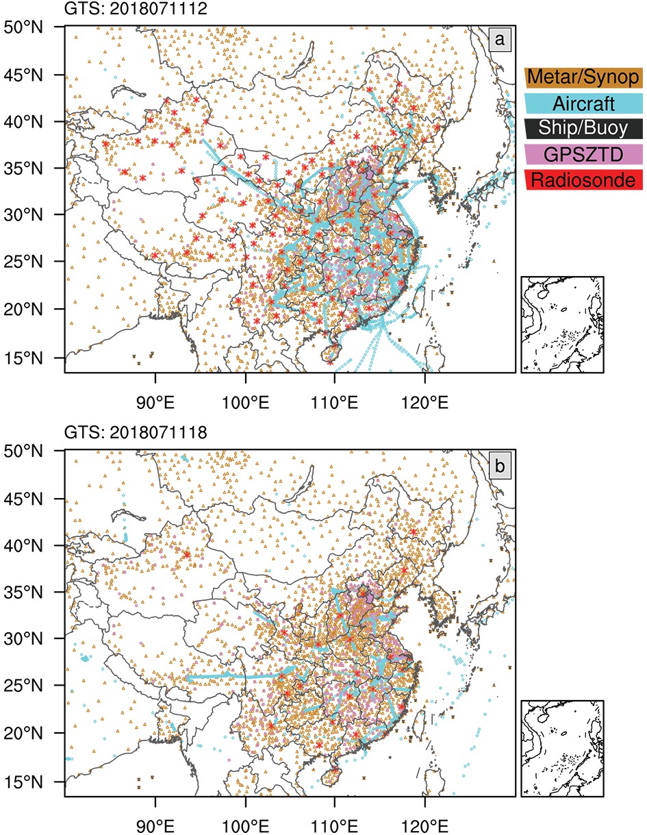 Figure1. Experimental domain and two typical examples of assimilated observations on (a) 1200 UTC July 11, 2018 and (b) 1800 UTC July 11, 2018.
The GM forecast data released by the European Centre for Medium-Range Weather Forecasts (ECMWF) (
2
2.2. Data assimilation
RMAPS-ST employs the 3DVAR algorithms from the WRF data assimilation (WRFDA, version-3.8.1) system (Barker et al., 2012). Following Sun and Wang (2013), five control variables are used for DA to reflect the convective systems development in the initial field: velocity components in the x- and y-directions, temperature, pseudo-relative humidity, and surface pressure. RMAPS-ST uses the National Meteorological Center (NMC) (Parrish and Derber, 1992) method to generate the background error covariance based on one-month forecasts in different seasons.RMAPS-ST assimilates various kinds of observations, including the upper-air wind, temperature, and specific humidity from radiosondes, aircraft reports and wind profilers. Surface wind, temperature, pressure, and specific humidity are obtained from land-based synoptic reports (SYNOP), aviation routine weather reports (METAR), and ship and buoy reports over the sea. Additionally, to improve the temporal and spatial distribution of the initial humidity in air columns, Global Positioning System Zenith Total Delay (GPSZTD) observations from over 500 sites in China are assimilated following quality control (Zhong et al., 2017). Note that not all of these assimilated observations are obtained regularly at every analysis time. For example, there are many more radiosonde observations at the conventional sounding time, i.e., 0000 and 1200 UTC, than at other times. There are also more aircraft reports during the daytime than at nighttime. Two typical distributions of the observations available for assimilation over China at 1200 UTC and 1800 UTC July 11, 2018, are shown in Fig. 1. The assimilation time-window for all observed data is ±1 h at each analysis time.
2
2.3. Dynamic blending
In the new FC strategy, DB blends the forecasts from ECMWF and WRF to form the first guess for DA. We use the blended field as the first guess for DA to provide a better background for DA than the WRF forecast itself from the previous cycle (?irokà et al. 2001; Gustafsson et al., 2018). Blending uses a Raymond sixth-order tangent low-pass filter to isolate the large-scale waveband from a limited area field x (labeled by


where


where


Two steps are implemented to determine the cutoff wavenumber in DB. The first is to select a large-scale waveband filtered by Eq. (1) from the ECMWF GM data. The waveband should be accurate enough as a candidate for blending. DB selects the GM large-scale waveband that has an acceptable bias tolerance at every level. The GM forecast biases are estimated (as a percentage) against the corresponding analysis by comparing their velocity difference in the form of kinetic energy


Since the ECMWF analysis cannot be obtained in real-time, the


The second step of DB aims to maintain the growth of small-scale systems in the initial fields at every level, because introducing too many GM waves would dampen the growth of small-scale modes in the RM fields (an extreme case is the “cold restart” run, in which the small-scale modes are regenerated from scratch). DB calculates the residual small-scale waveband kinetic energy difference (labeled


The small-scale waveband is also obtained using the Raymond filter as Eq. (1) shows. This study determines


3.1. Experimental design
Three batch experiments are performed for July 2018 (referred to as July cases) to compare the new FC strategy with both DA and DB (FC_DBDA), PC strategy with DA (PC_DA) and FC strategy with DA (FC_DA). The July cases cover seven-day 3-hour cycling runs for the period from 0000 UTC 11 July, 2018 to 2100 UTC 17 July, 2018 with a total of 56 forecast cycles. All experiments conduct a 6-hour WRF initialization to generate the initial fields in the first cycle and perform DA and a 24-hour WRF forecast in every cycle. FC_DA directly uses the 3-hour WRF forecast from the previous cycle as the first guess for DA (Fig. 2a). Experiment PC_DA is the same as FC_DA but reinitializes the forecast system from the ECMWF forecast once a day at 0000 UTC with a 6-hour spin-up process starting from the previous 1800 UTC (Fig. 2b, using the 1200 UTC+6 h EC forecast as the initial fields). FC_DBDA uses the blended fields of WRF and ECMWF forecasts as the first guess for DA at each cycle (Fig. 2c). In addition, since PC_DA does not assimilate observation during the spin-up process at 0000 UTC, we performed an additional experiment (FC_DBDA2, only performed for July cases) that is configured following FC_DBDA but generates the initial fields at 0000 UTC without DA at 1800 and 2100 UTC. The FC_DBDA shows similar performance to the FC_DBDA (Fig. S12?S16). Hence, we mainly compare the results of FC_DA, PC_DA and FC_DBDA.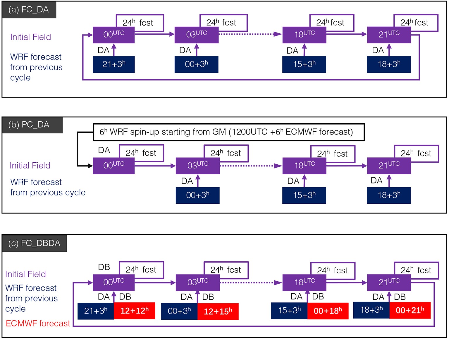 Figure2. Schematic of experiment FC_DA (a), PC_DA (b) and FC_DBDA (c) with a 3-hourly forecast cycle configuration. The WRF fields are the 3-hour forecasts from the previous cycle. The ECMWF fields are the forecasts at the same time starting from the previous 0000/1200 UTC.
FC_DBDA re-calculated the cutoff wavenumber


To verify the effectiveness of the new FC strategy in other seasons, we also perform the PC_DA and FC_DBDA experiments for three other seven-day periods: from 0000 UTC 11 Feb to 2100 UTC 17 Feb 2019 (referred to as February cases), from 0000 UTC 11 Apr to 2100 UTC 17 Apr 2019 (referred to as April cases), and from 0000 UTC 11 Oct to 2100 UTC 17 Oct 2019 (referred to as October cases). In these periods, we use the same parameter settings and cycle strategy as in the July cases. The experiments in these three seasons aim to investigate the applicability of the FC_DBDA strategy in RMAPS-ST. FC_DA is not included in these three periods because (1) the PC_DA strategy is the operational cycle strategy in the current version of RMAPS-ST, (2) the FC_DA cycle strategy has shown poorer performance than PC_DA in previous studies (Benjamin et al., 2016) and in July cases (see section 5), and (3) computer resources are limited for this study.
2
3.2. Verification metrics
We verify the performance of various forecast state variables, including u, v,


Quantitative precipitation forecasts are evaluated against observations from a national rain gauge network with more than 2600 sites over China (Fig. S3). We use two statistical indices to verify the precipitation forecasts - the Critical Success Index (CSI) and the Frequency BIAS (FBIAS) score. The rainfall events related to CSI and FBIAS are defined as precipitation amounts greater than or equal to a prescribed threshold such as 0.1, 1, 10, 25, and 50 mm.
The spin-up speed of the model is represented by the mean surface pressure tendency (MSPT, see Eq. (7) of Benjamin et al., 2004a) over the experimental domain, following many previous studies (Benjamin et al., 2004a; Wang et al., 2014; Vendrasco et al., 2016; Feng et al., 2020). A favorable RRC system should have low and smooth MSPT in the first few integrating hours to maintain model balance.
4.1. Verification of state variables
We first compare the multi-cycle averaged RMSE against upper-air observations for air temperature, specific humidity, u, and v. Figure 3 is the vertical profile of the RMSEs of initial fields (
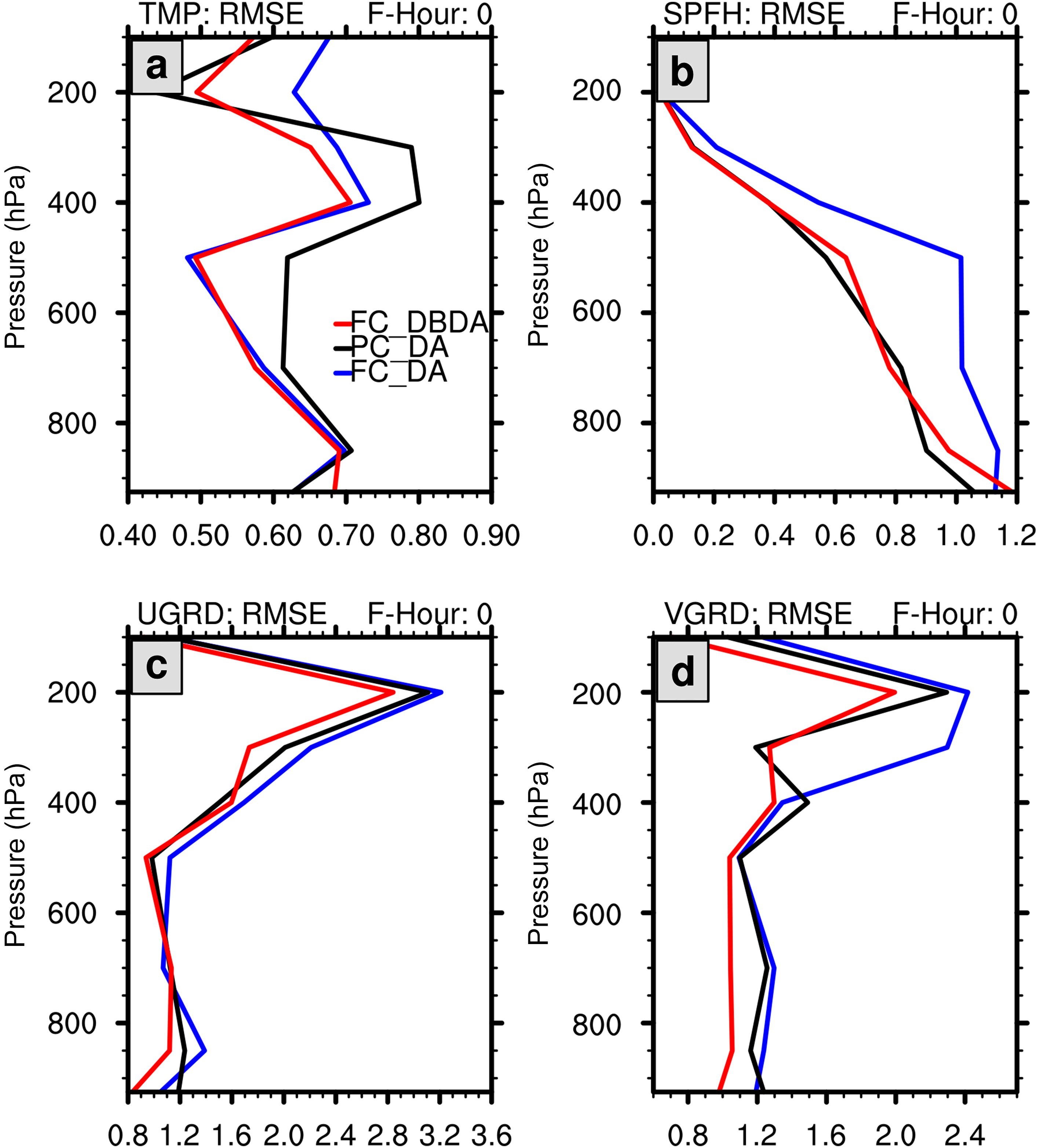 Figure3. Multicycle-averaged vertical profiles of initial RMSE (t = 0 h) over the experimental domain in July cases against real observations for (a) air temperature (units: K), (b) specific humidity (units: 10–1 g kg–1), (c) velocity component in x-direction u (units: m s–1), and (d) velocity component in y-direction v (units: m s–1). The blue, black, and red curves denote the RMSEs of FC_DA, PC_DA, and FC_DBDA, respectively.
 Figure4. Multicycle-averaged RMSE for 0–24 h forecasts over the experimental domain in July cases against real observations for (a) air temperature at 2 m (units: K), (b) surface pressure (units: hPa), (c) specific humidity at 2 m (units: g kg–1), and (d) wind speed at 10 m (units: m s–1). The blue, black, and red curves denote the RMSEs of FC_DA, PC_DA, and FC_DBDA, respectively.
We also verify the initial fields and 6 h and 24 h forecasts for the state variables using GFS final reanalysis data (Fig. S6–S8). Like the verification results against real observations, FC_DBDA shows the smallest initial and forecast RMSEs at almost all levels among the three experiments. The FC_DBDA mainly improves the temperature and wind at most levels and the humidity fields at mid-levels.
To examine the effects of different cycle strategies on WRF initial fields in detail, we also investigate the spatial patterns of initial bias for geopotential height at the 18th model level (~500 hPa) and specific humidity at the 12th model level (~700 hPa) (Fig. 5) over the experimental domain. The FC_DA shows the strong positive initial bias in geopotential height over central and eastern China and the negative bias over the south Tibetan Plateau and South Asia. The distribution of bias indicates an underestimation of the East Asian Trough (EAT) intensity, which is often located over eastern China and the western Pacific (e.g., Wang et al., 2009). Also, there is an overestimation of specific humidity over a belt from the Indochina Peninsula to northeast China, which is the main Moisture Transport Pathway (MTP) for summer precipitation in China (e.g., Zhao et al., 2016). Over the subtropical high region, i.e., the western Pacific, FC_DA underestimates the humidity. These results indicate that an RRC cannot rectify the large-scale errors only using DA. By contrast, PC_DA can rectify such bias to some degree due to the periodic restarting process from ECMWF forecasts, but the FC_DBDA improves the initial fields with better performance: most of the positive RMSEs of geopotential height over eastern China and specific humidity over the MTP are corrected. Consequently, the different effects of initial bias correction of the three strategies propagate to the forecast and generate similar bias patterns of state variables (Figs. S9 and S10), which would cause different performances in precipitation forecasts.
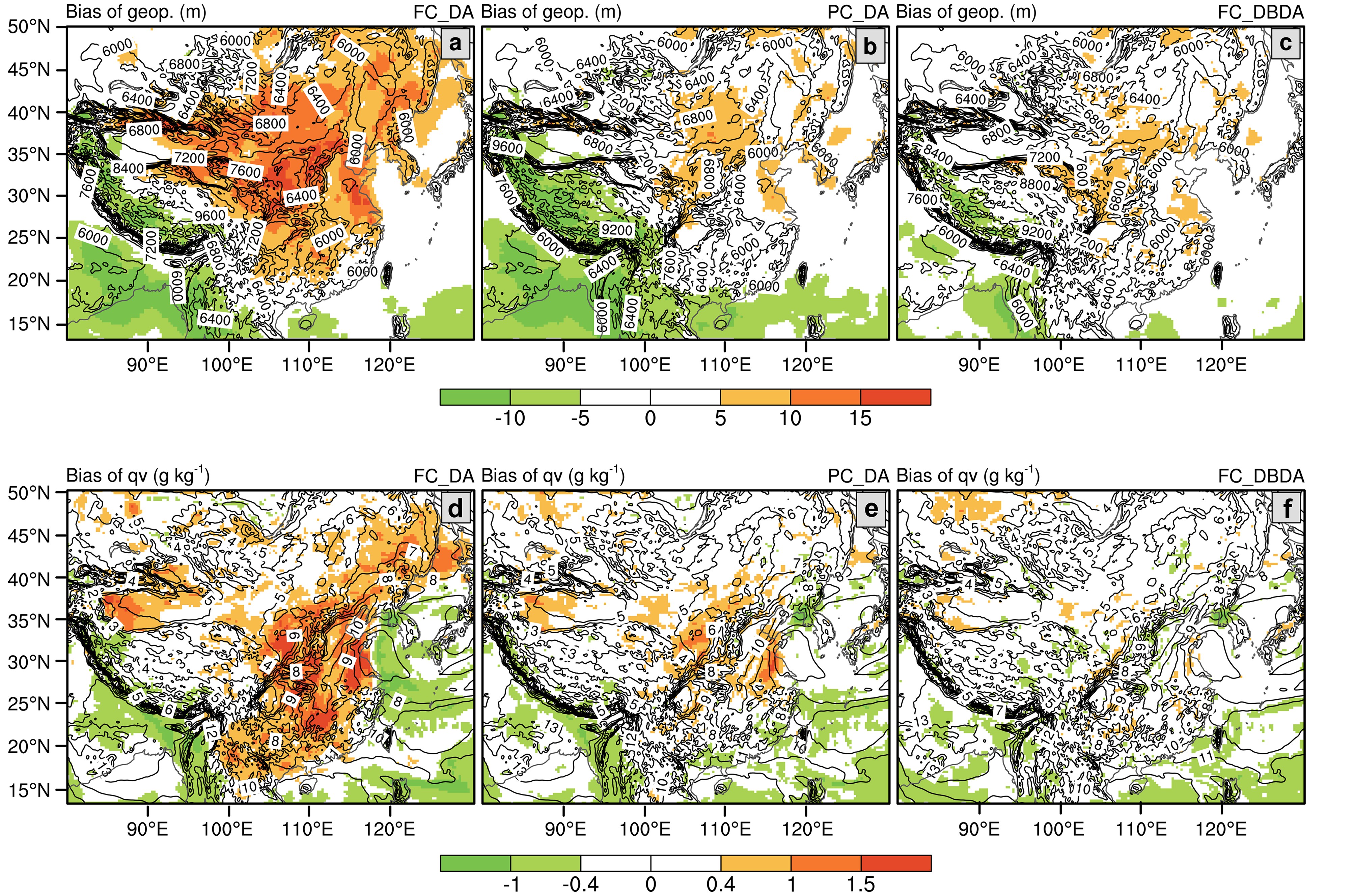 Figure5. Geographical distribution of multicycle-averaged initial field (contour lines) and initial bias (shaded) of geopotential height (units: m) (a, b, and c) at the 18th model level (~500 hPa) and of specific humidity (units: g kg–1) (d, e and f) at the 12th model level (~700 hPa) in July cases against GFS final reanalysis data for (a) and (d) FC_DA, (b) and (e) PC_DA, and (c) and (f) FC_DBDA respectively. All fields are preprocessed using 5-points smoothing to avoid the impact of horizontal resolution difference between WRF and GFS final reanalysis data.
2
4.2. Verification of precipitation forecasts
We use multi-cycle averaged CSI and FBIAS scores of 3-hour accumulated precipitation with the precipitation amount thresholds of 0.1, 1, 5, 10, 25, and 50 mm to evaluate the forecast skill of the three experiments (Fig. 6). For events with the 3-hour accumulated precipitation less than 0.1, 1, and 5 mm, the FC_DBDA has higher CSI and less FBIAS than the other two strategies. For the uncommon heavy rain events with 3-hour accumulated precipitation larger than 10, 25, and 50 mm, FC_DBDA has the highest CSI score in more than half the forecasts. Without large-scale constraints, modeled small-scale systems would develop much easier in FC_DA. As a result, FC_DA has better FBIAS scores for heavy rain events but worse CSI scores than the other two experiments. In contrast, FC_DBDA tends to depress the development of heavy precipitation events, which provide smoother control variables than FC_DA. To summarize, the FC_DBDA strategy has better precipitation forecast skills than FC_DA and PC_DA, especially for light to moderate precipitation events.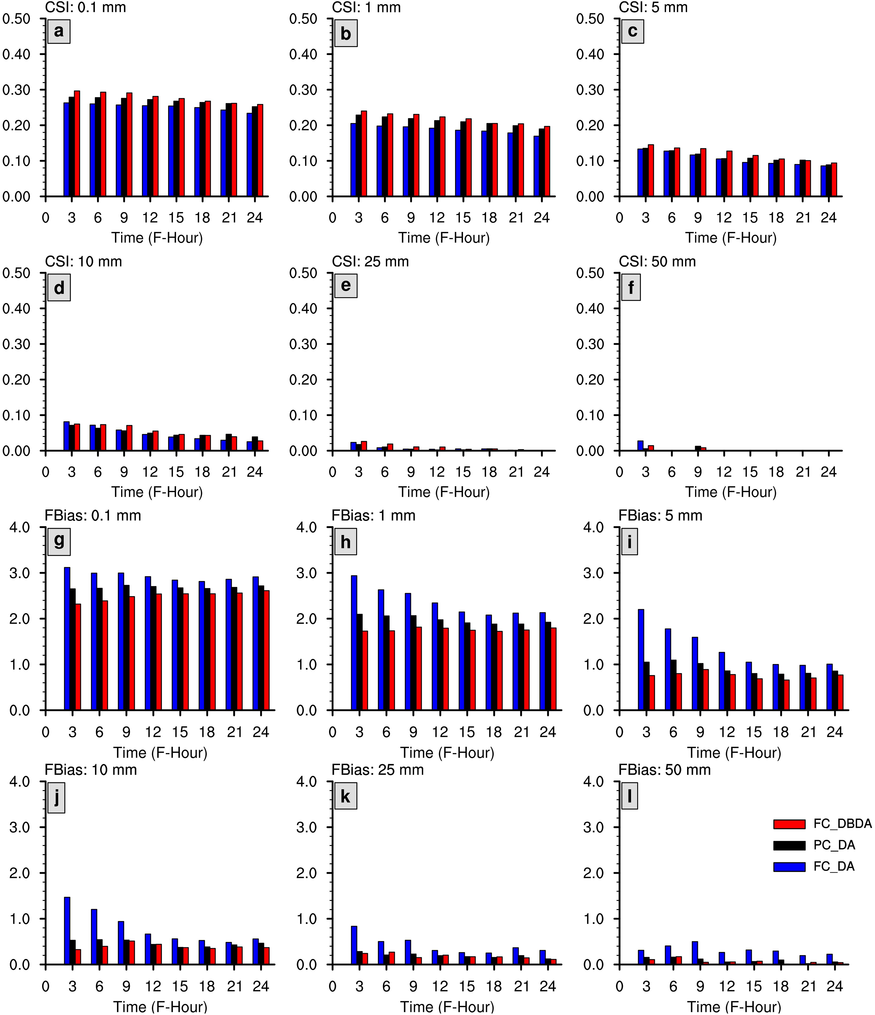 Figure6. Multicycle-averaged CSI (a–f) and FBIAS (g–l) scores of 3-h accumulated precipitation over the experimental domain in July cases for precipitation amount greater than or equal to 0.1, 1, 10, 25, and 50 mm. The blue, black, and red bars denote the scores of FC_DA, PC_DA, and FC_DBDA, respectively.
Figure 7 shows forecasts of time-averaged 24-hour accumulated precipitation, obtained by summing precipitation forecasts for the 5th–7th hour from all cycles. We compare the precipitation forecasts with the rain gauge data, which is interpolated to model grid cells using nearest neighbor interpolation. We only use the site observations within 9 km of every grid cell (i.e., length of 1 grid cell) to minimize the interpolation error. The FC_DBDA strategy results in precipitation patterns in closest agreement with the rain gauge observations. PC_DA experiments performed slightly better than FC_DA in the North China Plain (NCP) and South China (SC). Comparing with FC_DA and PC_DA, the FC_DBDA mitigates the over-predicted precipitation over the long rainfall belt from Northeast to Southwest China and the light rain areas in SC. In particular, FC_DBDA predicts the three small rainfall belts located in the NCP, which are not correctly reproduced by FC_DA and PC_DA experiments. Besides, FC_DBDA also favorably predicts the heavy rainfall over Hainan Island. These improvements in the FC_DBDA experiments are possibly related to the forecast reduction in humidity bias (Fig. 5 and Fig. S10). FC_DA and PC_DA overestimate the low-level humidity on the MTP from Northeast to Southwest China and trigger more spurious precipitation in these regions. In contrast, the accuracy of the humidity fields in FC_DBDA favors a better precipitation pattern.
 Figure7. Time-averaged accumulated 24-hour precipitation forecasts in July cases for observations from (a) rain gauges and (b–d) forecasts from (b) FC_DA, (c) PC_DA, (d) FC_DBDA experiments. The accumulated precipitation in these experiments is calculated from the sum of the 5th–7th hour precipitation forecasts in every cycle.
2
4.3. Model balance issues
We use the multicycle-averaged MSPT in the first six forecast hours to show the degree of model balance for FC_DA, FC_DBDA, and the spin-up process of PC_DA (Fig. 8). The results of cycles that start from non-0000/1200 UTC and those that start from 0000/1200 UTC cycles are presented separately because the ECMWF forecast used in RMAPS-ST restarts at 00/12 UTC (see section 2.1). Since the ECMWF forecast provides the LBCs and blended fields, such a change will slow down the model spin-up speed at 0000/1200 UTC relative to non-0000/1200 UTC (Fig. 8a).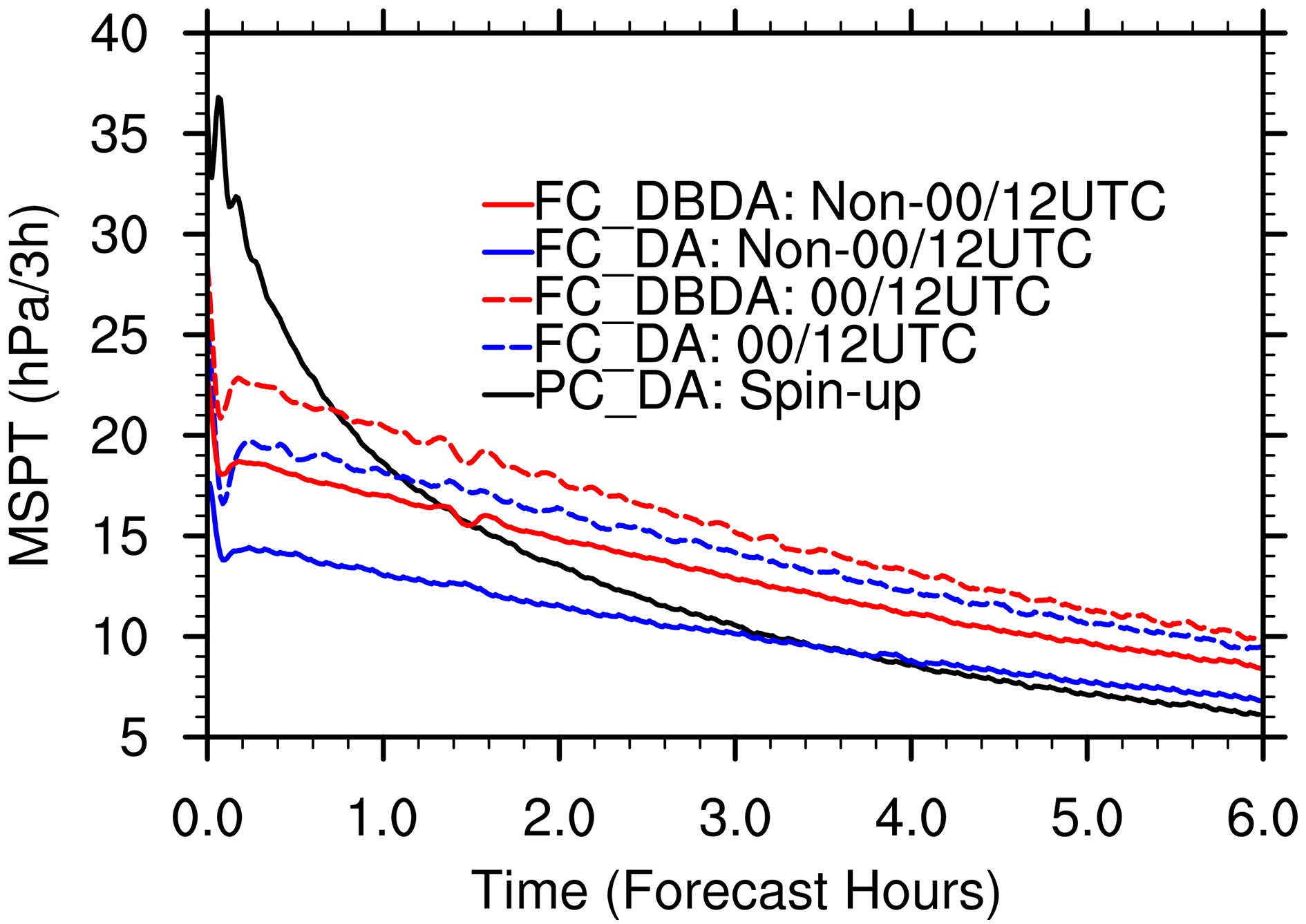 Figure8. Multicycle-averaged MSPT during the first 6 forecast hours for the July cases. The black, red, and yellow lines denote the results of the FC_DA, the spin-up process of PC_DA, and the FC_DBDA, respectively. The solid (dashed) lines denote the results of cycles that start from non-0000/1200 UTC (0000/1200 UTC) cycles for the two continuous cycle strategies.
The FC_DBDA strategy reaches model balance much faster than the spin-up process from the ECMWF forecasts used by PC_DA, since the FC_DBDA strategy includes the small-scale information from the WRF forecast in the previous cycle. The PC_DA strategy requires almost 2 hours of spin-up to achieve balance (Fig. 8b). Moreover, due to the DA adjustment, MSPT in FC_DA and FC_DBDA fluctuate sharply at the beginning of initialization but quickly become smooth after 20 minutes. Considering that the FC_DA only adjusts the initial fields using DA and the FC_DBDA strategy directly blends the longwave band of ECMWF forecasts into WRF without a cold-start process, FC_DBDA does add some noise to the initialization fields and has a slightly larger MSPT at the initial time than FC_DA. However, the MSPT curves of FC_DBDA are smooth, suggesting that the model balance is less affected by the FC_DBDA strategy and can be quickly re-adjusted within a short period. In addition to the MSPT, we found that the RMSE of surface pressure in FC_DBDA at the initial time and the first 3 hours is stable and smaller than in the other two experiments (Fig. 4b). The results also suggest that the model balance of the FC_DBDA strategy is acceptable in the RRC system.
2
4.4. Forecast continuity issue
To provide stable predictions for operational weather centers, the forecast precipitation pattern for a specific time should change little between two adjacent cycles. Here we explore the difference between the 3 h precipitation from the current cycle and the 6 h precipitation from the previous cycle in the three experiments (Fig. 9). The precipitation differences between adjacent cycles in FC_DBDA are smaller than in the FC_DA and PC_DA experiments in North China, Northeastern China and Central China. Considering that the RMAPS-ST focuses on the precipitation forecast in China, the results are acceptable. For precipitation over parts of southwest China and most marine areas, PC_DA and FC_DA are slightly better than FC_DBDA, which suggested that the dynamic blending process has few adverse effects on the forecast continuity of the precipitation pattern in other areas of the experimental domain.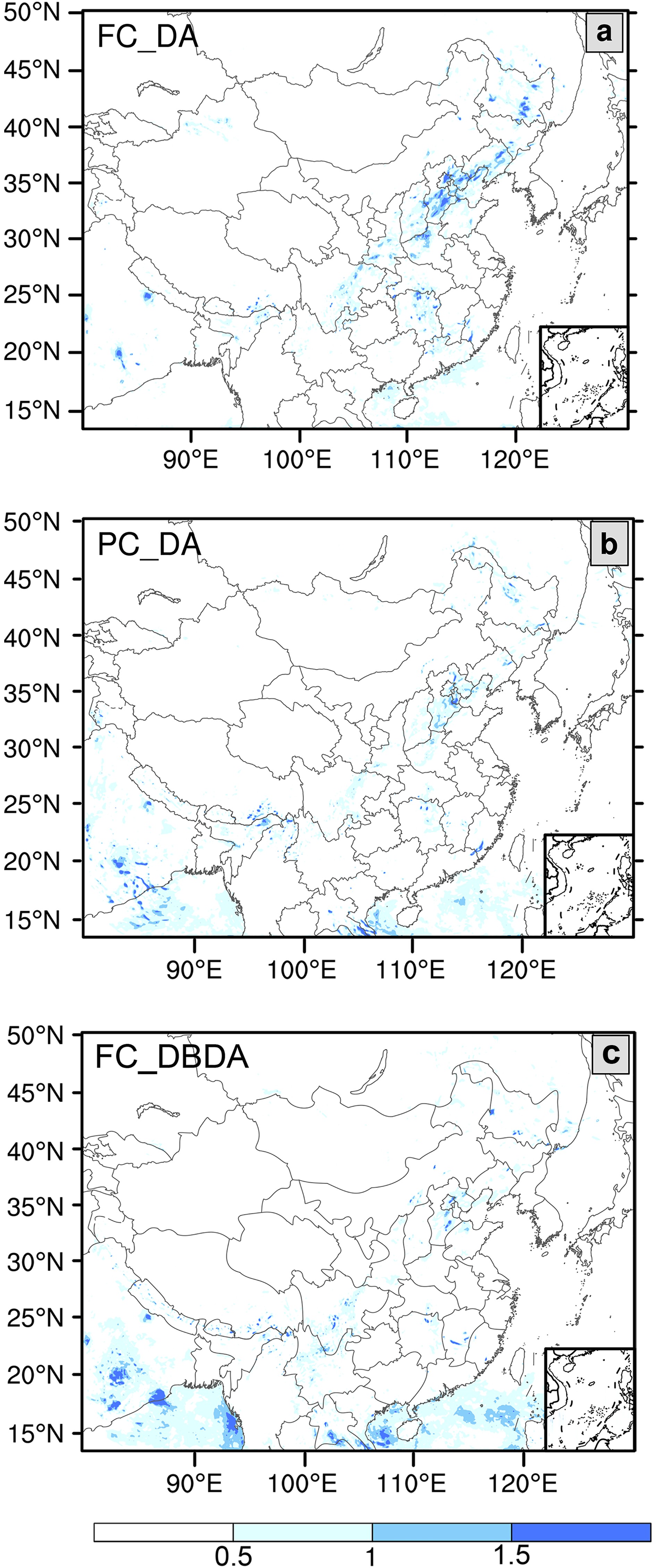 Figure9. Multicycle-averaged precipitation differences between the 3-h precipitation (mm) from the current cycle and the 6-h precipitation from the previous cycle in (b) FC_DA, (c) PC_DA, (d) FC_DBDA experiments.
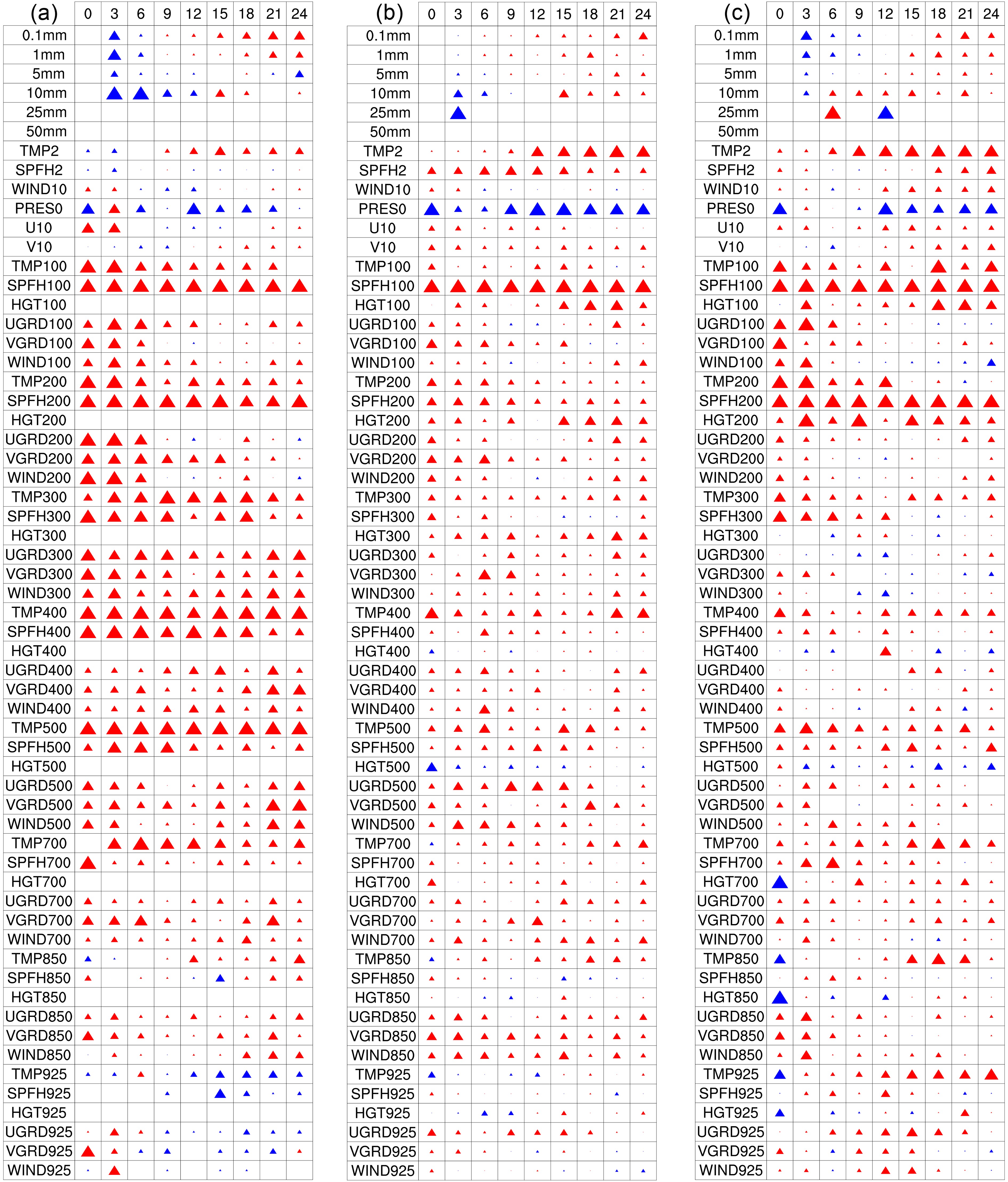 Figure10. Summary of the performance of FC_DBDA relative to PC_DA strategy for 3, 6, 9, 12, 15, 21, 24-hour forecasts from (a) February, (b) April, and (c) October cases. The red (blue) triangles indicate that the FC_DBDA (PC_DA) strategy performed better in at least 50% of forecasts than PC_DA (FC_DBDA). The size of the triangle is proportional to the “winning percentage” of the corresponding strategy. The quantified performances are calculated using CSI scores for various precipitation events and RMSEs for surface and upper-air state variables.
The new full-cycle strategy (FC_DBDA) was verified and compared with traditional partial cycle (PC_DA) and DA full cycle strategies (FC_DA) using the 3-hour cycle and the ECMWF forecasts as in RMAPS-ST. The 7-day period FC_DBDA experiments in July showed smaller initial and forecast biases than FC_DA and PC_DA for most verification variables. In particular, FC_DBDA corrected the large underestimation of geopotential height near the East Asian Trough and the overestimation of the intensity of the transport pathway of water vapor in summer over China. Consequently, the geographic rainfall pattern and the forecast skills on moderate and light rainfall were also significantly improved in FC_DBDA experiments. In addition, the model balance speed of FC_DBDA was less affected by the introduced large-scale waveband from ECMWF data due to the reserved small-scale information from the last cycle. The WRF re-balances the model fields within a short time, much faster than the spin-up process from ECMWF forecasts used by PC_DA. Moreover, the FC_DBDA improves the forecast continuity with smaller differences in precipitation patterns between two adjacent cycles.
To investigate the performance of the FC_DBDA relative to the currently used PC_DA in RMAPS-ST in other seasons, we further compared the forecast performance of FC_DBDA and PC_DA in three other periods, February, April and October, with similar 7-day and 3-hour-cycle batch experiments. The results show that the FC_DBDA improved the forecasts in most verification items in the three periods as in July. Hence, such a new full cycle strategy has the potential to replace the currently used partial cycle strategy in RRC.
It should be noted that the FC_DBDA strategy does not introduce more large-scale information than PC_DA at the cold-restart time (i.e., 0000 UTC) without regard for the error generated in the spin-up process. In comparison with the partial cycle, blending can ingest large-scale information with a negligible computing burden and acceptable model instability. Therefore, the improvements of FC_DBDA should be attributed to the continuously and easily ingested large-scale field during every cycle, which is poorly implemented by partial cycle in an operational RRC system.
Although the full cycle strategy with DA and DB has these considerable advantages, it should be noted that the new full cycle strategy has less impact on the forecasts of heavy rainfall, possibly because the direct blending process provides a dry atmospheric environment over the main transport pathway of water vapor in China (although it does correct the initial errors on humidity). Hence, accompanying its application in the new strategy, one should correspondingly adjust the physical schemes for moisture. Although this study does not use radar data assimilation, Ensemble Kalman Filter (EnKF), or hybrid variational-ensemble DA algorithms, considering the widely reported positive effects of radar reflectivity data assimilation (Sun et al., 2012; Tong et al., 2016) and these new ensemble-related DA algorithms (Schwartz and Liu, 2014; Schwartz et al., 2015) on the forecast of severe convection systems, we expect to improve the forecast skills for heavy rainfall with the new FC strategy.
Acknowledgements. We thank the helpful suggestions from Dr. J. SUN and the two anonymous reviewers. This work is supported by the National Key R&D Program of China (2018YFC1506803, 2019YFB2102901) and National Natural Science Foundation of China (Grant 41705135, 41790474).
Electronic supplementary material: Supplementary material is available in the online version of this article at
